- 原始文档: John E. Kerrigan(jkerriga@rutgers.edu, kerrigje@umdnj.edu) 3.3.1版本 4.6版本
- 参考译文: 梁(leunglm@hotmail.com)
- 2016-08-10 15:39:10 增加gmx-5.x版本命令, 由 汪洋 测试提供
- 2016-09-02 11:36:18 感谢 陈孙妮 修订翻译舛误之处.
概述
在本教程中, 你将研究一种从漏斗网蜘蛛的毒液中分离出来的毒素. 毒液毒素在以前一直被用于识别阳离子通道. 钙离子通道会调节进入细胞的钙离子. 神经信号受到神经细胞中离子平衡的高度控制. 人们认为像蜘蛛毒素这类毒液中暴露的带正电残基会倾向于与细胞离子通道入口的带负电残基结合. 对本教程中的蜘蛛毒素, 其带正电的残基主要朝向肽链一侧. 离子通道的堵塞会导致神经信号的中断, 导致麻痹并最终死亡(通过呼吸衰竭推测).
GROMACS是一个利用经典分子动力学理论研究蛋白质动力学的高端高效工具[1,2], 它是遵守GNU公共许可的自由软件, 你可以从GROMACS官方网站下载. GROMACS可以在linux, unix和Windows上运行. 对于本教程, 我们使用的是GROMACS 4.6版, 并给出了5.x版本相应的命令. 编译时使用了3.3.3版本的FFTW库.
在本教程中, 你要创建GROMACS结构文件(*.gro), 可使用VMD, visual molecular dynamics查看这种文件. 另外, 你还需要一份GROMACS用户手册.
本教程关注的蛋白质来自下面的文献:
Yu, H., Rosen, M. K., Saccomano, N. A., Phillips, D., Volkmann, R. A., Schreiber, S. L.: Sequential assignment and structure determination of spider toxin omega-Aga-IVB. Biochemistry 32 pp. 13123 (1993)
我们将使用显式的溶剂动力学研究这个肽毒素. 我们首先会将这个小肽放于水盒子中进行溶剂化, 然后利用牛顿运动定律进行平衡. 我们还将比较和对比补偿离子对显式溶剂动力学的影响. 通过模拟, 我们希望能回答如下几个问题:
- 小肽的二级结构和三级结构在动力学模拟中是否稳定?
- 带正电的残基侧链是否主要朝向肽结构的一侧?
- 补偿离子是保持在正电残基附近还是四处移动?
- 水在维持蛋白结构中起到什么作用?
分子动力学模拟
理解预平衡
如果你研究过不同的MD教程, 就会发现在进行成品模拟前, 不同教程的处理存在差异. 不了解的人就会觉得困惑. 所以我们要知道原则, 这样才能知道为什么会有不同的处理方法.
在做成品MD模拟前, 最好保证体系已经达到平衡, 因为我们最终目的是对平衡好的体系进行抽样. 如果体系没有平衡好, 那么需要先运行很长时间的模拟达到平衡, 然后才能采集数据. 为了使模拟开始时的体系尽量接近平衡, 可以采取各种方法, 这些方法可以统称为预平衡.
可见, 预平衡并不是必须的. 如果体系的初始结构足够好, 就不需要特别的预平衡, 直接做模拟即可. 分析结果时将模拟的前面一部分作为预平衡过程舍去即可. 但当体系的初始结构不是很好时, 达到平衡可能耗时较长. 对一些很差的初始结构, 模拟可能会崩溃, 这种情况下, 就需要根据具体情况采用一些预平衡方法.
-
蛋白质结构能量最小化 因为pdb文件中的蛋白质结构来自晶体, 里面可能含有溶剂分子, 各种离子. 这样的结构可能与真空中的结构有差距, 也可能与溶液中的结构有差距. 如果要对溶液中蛋白质进行模拟, 可以先对蛋白质进行溶液中的能量最小化. 因为能量最小化可以比较迅速地将结构调整至能量较低的构型, 这样MD的时候就可以比较快地达到平衡了, 相对节约了时间. 如果模拟体系中还含有离子, 也可以添加离子和溶剂后再进行能量最小化.
-
蛋白质位置限制性模拟 有时添加溶剂分子和离子后, 体系中有些原子之间距离过近, 相互之间的作用力过大, 模拟时可能会导致蛋白质结构散掉甚至体系崩溃. 为避免此类问题, 可以先对蛋白质进行位置限制性模拟, 通过限制蛋白质中的重原子, 维持其结构. 等溶剂分子, 离子的位置调整好了之后再放开蛋白质分子的位置限制进行模拟.
-
NVT预平衡 做NPT模拟时盒子大小会改变, 如果初始体系内压力太大, 盒子可能改变太大, 从而引起体系崩溃. 为此, 先进行NVT模拟减小盒子的内压力, 再用NVT平衡好的结构作为初始结构进行NPT模拟可能会解决崩溃问题.
上面的三种方法可以根据具体情况选用, 也可以联合起来使用. 在这个教程中, 使用的预平衡方法就是能量最小化 -> 位置限制性NVT -> 位置限制性NPT. 其实, 如果蛋白质结构比较稳定, 只使用位置限制性NPT模拟作为预平衡也可以. 但为了保险起见, 还是建议至少使用能量最小化 -> 位置限制性NPT.
第一步: 获取并处理pdb文件
从Protein Data Bank下载小肽的pdb文件1OMB.PDB(或点击这里下载). 在Linux下你可使用如下命令:
wget http://www.rcsb.org/pdb/files/1OMB.pdb
下面是这个小肽的二级结构示意图.
在用GROMACS的程序对pdb文件进行处理前, 要做许多检查, 以保证pdb文件的完整性. 根据pdb文件的不同, 要进行不同的处理. 需要处理的方面包括但不限于:
- 氢原子
- C端氧原子
- 结晶水
- 缺失原子/残基/侧链
- 二硫键
- 带电残基
这些都需要你熟悉pdb文件的格式, 并知道一些常用的处理pdb文件的工具.
如果你知道下载的结构可能有混乱(例如, 残基有缺失的侧链), 建议先用DeepView软件预览一下下载的文件. DeepView可以替换缺失的侧链(但是, 注意DeepView可能会在添加的侧链前加上奇怪的控制字符, 而且这些符号只能在文本编辑器中手工去掉!). 在我们下载的这个pdb文件不存在缺失的侧链, 我们就不必担心了.
但是, 我们下载的pdb文件中缺少C端的结束氧原子, 需要在C端结束处添加氧原子类型OXT. 操作步骤如下:
- 在DeepView中打开
1OMB.pdb(或在unix shell中键入spdbv 1OMB.pdb) - 菜单
Build->Add C-terminal Oxygen (OXT), DeepView会删除氢原子并添加缺失的氧原子. - 菜单
File->Save->Current Layer将文件保存为fws.pdb.
使用文本编辑器检查得到的fws.pdb文件, 保证HEADER和COMPND行具有名称(实际上, 任何名称都可以), 删除DeepView添加到文件末尾的以SPDBV开头的行.
处理后的fws.pdb文件见这里. 和原先的1OMB.PDB文件相比, 可以看到fws.pdb文件中已经不含氢原子, 删除了SEQRES, SHEET, SSBOND, CONECT信息, 并且添加了OXT原子.
说明: 无论何时将一个文本文件从Windows系统复制到unix系统, 一定要转换成unix文本文件. 像MS Word这类Windows编辑器会在文件中加入控制符, 这可能会使unix程序产生错误. 你可以用to_unix命令(如to_unix filename filename将filename文件转换成unix文本文件. 在RedHat Linux中, 还可以使用dos2unix命令.)
第二步: 用pdb2gmx获得拓扑文件
pdb2gmx命令(使用pdb2gmx -h查看选项; 其实可以用-h选项查看所有GROMACS命令的帮助文档)可利用pdb文件创建GROMACS的输入坐标和拓扑文件. 拓扑文件包含了所有力场参数(基于所选择的力场), 因此非常重要.
gmx-4.x: pdb2gmx -ignh -ff amber99sb-ildn -f fws.pdb -o fws.gro -p fws.top -water tip3p
gmx-5.x: gmx pdb2gmx -ignh -ff amber99sb-ildn -f fws.pdb -o fws.gro -p fws.top -water tip3p
-ignh: 忽略输入pdb文件中的所有氢原子. 因为本pdb文件是由NMR产生的, 含有氢原子, 所以用此选项忽略文件中的氢原子, 统一使用GROMOS力场的氢原子命名规则, 以免出现氢原子名称不一致的情况.-ff: 指定使用的力场. 我们使用Amber99SB-ILDN力场[3]. 也可以使用其他力场, 请根据自己的体系进行选择.-f: 指定需要进行处理的蛋白质结构文件-o: 指定一个新生成的GROMACS文件名(也可以是其它的文件类型, 如pdb)-p: 指定新生成的拓扑文件名, 包含所有原子及原子间的相互作用参数-water: 指定水模型. 我们使用TIP3P水模型[4]. 也可以使用其他水模型, 如SPC/E[5], 请根据自己的需要选择.
命令运行成功, 打印出下面的说明(gmx-4.x):
Using the Amber99sb-ildn force field in directory C:/Users/Jicun/E_Prf/Gromacs-4.6/share/top/amber99sb-ildn.ff

Opening force field file C:/Users/Jicun/E_Prf/Gromacs-4.6/share/top/amber99sb-ildn.ff\aminoacids.r2b
Opening force field file C:/Users/Jicun/E_Prf/Gromacs-4.6/share/top/amber99sb-ildn.ff\dna.r2b
Opening force field file C:/Users/Jicun/E_Prf/Gromacs-4.6/share/top/amber99sb-ildn.ff\rna.r2b
Reading fws.pdb...
Read 'OMEGA-AGA-IVB', 257 atoms
Analyzing pdb file
Splitting chemical chains based on TER records or chain id changing.
There are 1 chains and 0 blocks of water and 38 residues with 257 atoms

  chain  #res #atoms
  1 'A'    35    257

All occupancies are one
Opening force field file C:/Users/Jicun/E_Prf/Gromacs-4.6/share/top/amber99sb-ildn.ff\atomtypes.atp
Atomtype 1
Reading residue database... (amber99sb-ildn)
Opening force field file C:/Users/Jicun/E_Prf/Gromacs-4.6/share/top/amber99sb-ildn.ff\aminoacids.rtp
Residue 93
Sorting it all out...
Opening force field file C:/Users/Jicun/E_Prf/Gromacs-4.6/share/top/amber99sb-ildn.ff\dna.rtp
Residue 109
Sorting it all out...
Opening force field file C:/Users/Jicun/E_Prf/Gromacs-4.6/share/top/amber99sb-ildn.ff\rna.rtp
Residue 125
Sorting it all out...
Opening force field file C:/Users/Jicun/E_Prf/Gromacs-4.6/share/top/amber99sb-ildn.ff\aminoacids.hdb
Opening force field file C:/Users/Jicun/E_Prf/Gromacs-4.6/share/top/amber99sb-ildn.ff\dna.hdb
Opening force field file C:/Users/Jicun/E_Prf/Gromacs-4.6/share/top/amber99sb-ildn.ff\rna.hdb
Opening force field file C:/Users/Jicun/E_Prf/Gromacs-4.6/share/top/amber99sb-ildn.ff\aminoacids.n.tdb
Opening force field file C:/Users/Jicun/E_Prf/Gromacs-4.6/share/top/amber99sb-ildn.ff\aminoacids.c.tdb
Processing chain 1 'A' (257 atoms, 35 residues)
Identified residue CYS4 as a starting terminus.
Identified residue PRO38 as a ending terminus.
8 out of 8 lines of specbond.dat converted successfully
Special Atom Distance matrix:
					CYS4   CYS12   CYS19   CYS20   CYS25   CYS27   MET29
					 SG6    SG67   SG118   SG124   SG163   SG180   SD193
   CYS12    SG67   1.202
   CYS19   SG118   0.727   0.705
   CYS20   SG124   0.202   1.267   0.730
   CYS25   SG163   1.159   0.202   0.570   1.197
   CYS27   SG180   1.813   0.627   1.223   1.854   0.666
   MET29   SD193   2.596   1.490   1.906   2.622   1.466   0.949
   CYS34   SG227   1.742   0.540   1.200   1.804   0.636   0.202   1.079
   CYS36   SG242   0.928   0.645   0.202   0.930   0.478   1.089   1.718
				   CYS34
				   SG227
   CYS36   SG242   1.085
Linking CYS-4 SG-6 and CYS-20 SG-124...
Linking CYS-12 SG-67 and CYS-25 SG-163...
Linking CYS-19 SG-118 and CYS-36 SG-242...
Linking CYS-27 SG-180 and CYS-34 SG-227...
Opening force field file C:/Users/Jicun/E_Prf/Gromacs-4.6/share/top/amber99sb-ildn.ff\aminoacids.arn
Opening force field file C:/Users/Jicun/E_Prf/Gromacs-4.6/share/top/amber99sb-ildn.ff\dna.arn
Opening force field file C:/Users/Jicun/E_Prf/Gromacs-4.6/share/top/amber99sb-ildn.ff\rna.arn
Checking for duplicate atoms....
Generating any missing hydrogen atoms and/or adding termini.
Now there are 35 residues with 495 atoms
Making bonds...
Number of bonds was 504, now 503
Generating angles, dihedrals and pairs...
Before cleaning: 1314 pairs
Before cleaning: 1356 dihedrals
Keeping all generated dihedrals
Making cmap torsions...There are 1356 dihedrals,   99 impropers,  906 angles
		  1308 pairs,      503 bonds and     0 virtual sites
Total mass 3798.434 a.m.u.
Total charge 2.000 e
Writing topology

Writing coordinate file...
				--------- PLEASE NOTE ------------
You have successfully generated a topology from: fws.pdb.
The Amber99sb-ildn force field and the tip3p water model are used.
				--------- ETON ESAELP ------------

gcq#37: "Never Get a Chance to Kick Ass" (The Amps)
我们得到了三个输出文件: 结构文件fws.gro, 拓扑文件fws.top, 位置限制文件posre.itp.
说明: 如果不在命令中使用-ff指定力场, 运行命令后会给出一个列表, 让你选择力场, 直接键入你要使用的力场编号再回车即可.
第三步: 创建模拟盒子
接下来我们使用editconf命令来创建周期性的模拟盒子.
gmx-4.x: editconf -f fws.gro -o fws-PBC.gro -bt dodecahedron -d 1.2
gmx-5.x: gmx editconf -f fws.gro -o fws-PBC.gro -bt dodecahedron -d 1.2
-f: 输入蛋白结构-o: 输出带模拟盒子信息的结构文件-bt: 默认使用长方盒子, 可以使用-bt选项改变盒子类型, 如八面体, 十二面体等-d: 蛋白与模拟盒子在X, Y, Z方向上的最小距离
我们使用-bt选项创建了一个菱形十二面体盒子, 因为这种盒子是接近球形, 计算效率最高. -d选项设定分子到盒子边缘的最小距离, 以nm为单位, 它决定了盒子的尺寸. 理论上在绝大多数系统中, -d都不能小于0.9 nm[6], 我们使用了1.2 nm.
命令运行成功, 打印出下面的说明(gmx-4.x):
Read 495 atoms
Volume: 0.001 nm^3, corresponds to roughly 0 electrons
No velocities found
	system size :  2.793  1.951  2.502 (nm)
	diameter    :  3.319               (nm)
	center      : -0.156 -2.386 -0.412 (nm)
	box vectors :  0.100  0.100  0.100 (nm)
	box angles  :  90.00  90.00  90.00 (degrees)
	box volume  :   0.00               (nm^3)
	shift       :  4.445  6.675  2.434 (nm)
new center      :  4.289  4.289  2.022 (nm)
new box vectors :  5.719  5.719  5.719 (nm)
new box angles  :  60.00  60.00  90.00 (degrees)
new box volume  : 132.24               (nm^3)

gcq#178: "Whatever Happened to Pong ?" (F. Black)
我们得到了置于周期性菱形盒子中的蛋白质分子.
说明: editconf也可以用于GROMACS文件(*.gro)和pdb文件(*.pdb)的相互转换. 例如: editconf -f file.gro -o file.pdb 可以将file.gro转换为file.pdb
第四步: 蛋白质分子真空中的能量最小化
现在就可以使用产生的文件进行 真空中的 能量最小化了. 若你只需要进行真空中的模拟, 完成此步骤后直接跳到成品模拟步骤即可.
GROMACS使用特殊的*.mdp文件指定每种计算类型的参数. 下面是em-vac-pme.mdp文件的内容:
| em-vac-pme.mdp | |
|---|---|
1 2 3 4 5 6 7 8 9 10 11 12 13 14 15 16 17 18 19 20 21 | ; 传递给预处理器的一些定义
define = -DFLEXIBLE ; 使用柔性水模型而非刚性模型, 这样最陡下降法可进一步最小化能量
; 模拟类型, 结束控制, 输出控制参数
integrator = steep ; 指定使用最陡下降法进行能量最小化. 若设为`cg`则使用共轭梯度法
emtol = 500.0 ; 若力的最大值小于此值则认为能量最小化收敛(单位kJ mol^-1^ nm^-1^)
emstep = 0.01 ; 初始步长(nm)
nsteps = 1000 ; 在能量最小化中, 指定最大迭代次数
nstenergy = 1 ; 能量写出频率
energygrps = System ; 要写出的能量组
; 近邻列表, 相互作用计算参数
nstlist = 1 ; 更新近邻列表的频率. 1表示每步都更新
ns_type = grid ; 近邻列表确定方法(simple或grid)
coulombtype = PME ; 计算长程静电的方法. PME为粒子网格Ewald方法, 还可以使用cut-off
rlist = 1.0 ; 短程力近邻列表的截断值
rcoulomb = 1.0 ; 长程库仑力的截断值
vdwtype = cut-off ; 计算范德华作用的方法
rvdw = 1.0 ; 范德华距离截断值
constraints = none ; 设置模型中使用的约束
pbc = xyz ; 3维周期性边界条件
|
对于其中的截断值的设置, 可参考下面的表格
| 力场 | 近邻列表 | 静电截断 | PME格点 | VdW类型 | VdW截断 | 必须使用DispCorr |
|---|---|---|---|---|---|---|
| GROMACS-UA | 1.0 | 1.0 | 0.135 | Shift | 0.9 | 是 |
| Cut-off | 1.4 | 否 | ||||
| OPLS-AA | 0.9 | 0.9 | 0.125 | Shift | 0.8 | 是 |
| Cut-off | 1.4 | 否 |
注意, 上表中shift/cutoff的单位为nm, UA=united atom, AA=all-atom, DispCorr只能和周期性边界条件一起使用.
GROMACS预处理器grompp(即gromacs pre-processor的缩写)可以将模拟参数, 分子结构, 所需要的力场参数等所有信息整合在一个单一的二进制文件(tpr文件)中, 运行mdrun时只需要tpr文件.
gmx-4.x: grompp -f em-vac-pme.mdp -c fws-PBC.gro -p fws.top -o em-vac.tpr
gmx-5.x: gmx grompp -f em-vac-pme.mdp -c fws-PBC.gro -p fws.top -o em-vac.tpr
-f选项指定输入参数文件, -c选项指定输入结构文件, -p选项指定输入拓扑文件, -o选项指定输出用于mdrun的输入文件.
运行命令, 屏幕输出(gmx-4.x)
Generated 2211 of the 2211 non-bonded parameter combinations
Generating 1-4 interactions: fudge = 0.5
Generated 2211 of the 2211 1-4 parameter combinations
Excluding 3 bonded neighbours molecule type 'Protein_chain_A'

NOTE 1 [file fws.top, line 4775]:
  System has non-zero total charge: 2.000000
  Total charge should normally be an integer. See
  http://www.gromacs.org/Documentation/Floating_Point_Arithmetic
  for discussion on how close it should be to an integer.

Analysing residue names:
There are:    35    Protein residues
Analysing Protein...
Number of degrees of freedom in T-Coupling group rest is 1482.00
Calculating fourier grid dimensions for X Y Z
Using a fourier grid of 48x48x48, spacing 0.119 0.119 0.119
Estimate for the relative computational load of the PME mesh part: 0.83

NOTE 2 [file em-vac-pme.mdp]:
  The optimal PME mesh load for parallel simulations is below 0.5
  and for highly parallel simulations between 0.25 and 0.33,
  for higher performance, increase the cut-off and the PME grid spacing.

This run will generate roughly 1 Mb of data

There were 2 notes

gcq#75: "Hold On Like Cliffhanger" (Urban Dance Squad)
gmx-5.x
NOTE 1 [file em-vac-pme.mdp, line 22]:
  em-vac-pme.mdp did not specify a value for the .mdp option
  "cutoff-scheme". Probably it was first intended for use with GROMACS
  before 4.6. In 4.6, the Verlet scheme was introduced, but the group
  scheme was still the default. The default is now the Verlet scheme, so
  you will observe different behaviour.
NOTE 2 [file em-vac-pme.mdp]:
  With Verlet lists the optimal nstlist is >= 10, with GPUs >= 20. Note
  that with the Verlet scheme, nstlist has no effect on the accuracy of
  your simulation.

Setting the LD random seed to 108284530
Generated 2211 of the 2211 non-bonded parameter combinations
Generating 1-4 interactions: fudge = 0.5
Generated 2211 of the 2211 1-4 parameter combinations
Excluding 3 bonded neighbours molecule type 'Protein_chain_A'
NOTE 3 [file fws.top, line 4771]:
  System has non-zero total charge: 2.000000
  Total charge should normally be an integer. See
  http://www.gromacs.org/Documentation/Floating_Point_Arithmetic
  for discussion on how close it should be to an integer.
  Removing all charge groups because cutoff-scheme=Verlet
Analysing residue names:
There are:    35    Protein residues
Analysing Protein...
Number of degrees of freedom in T-Coupling group rest is 1482.00
Calculating fourier grid dimensions for X Y Z
Using a fourier grid of 48x48x48, spacing 0.119 0.119 0.119
Estimate for the relative computational load of the PME mesh part: 0.85
NOTE 4 [file em-vac-pme.mdp]:
  The optimal PME mesh load for parallel simulations is below 0.5
  and for highly parallel simulations between 0.25 and 0.33,
  for higher performance, increase the cut-off and the PME grid spacing.
This run will generate roughly 1 Mb of data
There were 4 notes
gcq#553: "Should we force science down the throats of those that have no taste for it? Is it our duty to drag them kicking and screaming into the twenty-first century? I am afraid that it is." (George Porter)
得到运行输入文件em-vac.tpr, 参数文件mdout.mdp.
使用mdrun命令运行能量最小化
gmx-4.x: mdrun -v -deffnm em-vac
gmx-5.x: gmx mdrun -v -deffnm em-vac
-deffnm指定默认的文件名称, -v显示模拟过程中的信息.
经过98步, 计算结束(gmx-4.x)
Reading file em-vac.tpr, VERSION 4.6.2-dev (single precision)
Using 4 MPI threads
Compiled acceleration: SSE4.1 (Gromacs could use AVX_256 on this machine, which is better)

Steepest Descents:
   Tolerance (Fmax)   = 5.00000e+002
   Number of steps    =         1000
Step=    0, Dmax= 1.0e-002 nm, Epot= 1.41200e+003 Fmax= 5.70923e+003, atom= 150
Step=    1, Dmax= 1.0e-002 nm, Epot= -2.24422e+002 Fmax= 4.54461e+003, atom= 164
Step=    3, Dmax= 6.0e-003 nm, Epot= -7.68675e+002 Fmax= 3.09902e+003, atom= 150
Step=    4, Dmax= 7.2e-003 nm, Epot= -7.84120e+002 Fmax= 5.49768e+003, atom= 164
Step=    5, Dmax= 8.6e-003 nm, Epot= -8.30759e+002 Fmax= 5.95529e+003, atom= 164
......
Step=   98, Dmax= 2.1e-003 nm, Epot= -1.77253e+003 Fmax= 3.70245e+002, atom= 494

writing lowest energy coordinates.

Steepest Descents converged to Fmax < 500 in 99 steps
Potential Energy  = -1.7725271e+003
Maximum force     = 3.7024463e+002 on atom 494
Norm of force     = 7.0873062e+001

gcq#313: "My Brothers are Protons (Protons!), My Sisters are Neurons (Neurons)" (Gogol Bordello)
gmx-5.x
Running on 1 node with total 2 cores, 4 logical cores
Hardware detected:
  CPU info:
    Vendor: GenuineIntel
    Brand:  Intel(R) Core(TM) i5-4210U CPU @ 1.70GHz
    SIMD instructions most likely to fit this hardware: AVX2_256
    SIMD instructions selected at GROMACS compile time: SSE2
Compiled SIMD instructions: SSE2, GROMACS could use AVX2_256 on this machine, which is better
Reading file em-vac.tpr, VERSION 5.1.2 (single precision)
Using 1 MPI thread
Using 4 OpenMP threads
Steepest Descents:
   Tolerance (Fmax)   =  5.00000e+02
   Number of steps    =         1000
Step=    0, Dmax= 1.0e-02 nm, Epot=  1.45219e+03 Fmax= 5.70926e+03, atom= 150
Step=    1, Dmax= 1.0e-02 nm, Epot= -1.83565e+02 Fmax= 4.54459e+03, atom= 164
Step=    3, Dmax= 6.0e-03 nm, Epot= -7.28101e+02 Fmax= 3.09905e+03, atom= 150
Step=    4, Dmax= 7.2e-03 nm, Epot= -7.40962e+02 Fmax= 5.49785e+03, atom= 164
Step=    5, Dmax= 8.6e-03 nm, Epot= -7.86727e+02 Fmax= 5.95532e+03, atom= 164
......
Step=   98, Dmax= 2.1e-03 nm, Epot= -1.73279e+03 Fmax= 3.70232e+02, atom= 494
writing lowest energy coordinates.
Steepest Descents converged to Fmax < 500 in 99 steps
Potential Energy  = -1.7327905e+03
Maximum force     =  3.7023245e+02 on atom 494
Norm of force     =  7.0877754e+01
gcq#189: "It's So Fast It's Slow" (F. Black)
我们得到了日志文件em-vac.log, 全精度轨迹文件em-vac.trr, 能量文件em-vac.edr, 能量最小化后的结构文件em-vac.gro.
说明: 如果最小化不收敛, 可以将nsteps的数值增大再重新提交一次. 要重新提交作业的话, 你需要重新运行grompp.
第五步: 向盒子中填充溶剂及离子并进行能量最小化
gmx-4.x版本的genbox命令可以向给定尺寸/类型的周期性盒子中填充恰当数目的溶剂水分子. 在gmx-5.x版本中这个命令被分为gmx solvate和gmx insert-molecules两个命令. 但其使用方法类似.
gmx-4.x: genbox -cp em-vac.gro -cs spc216.gro -p fws.top -o fws-b4ion.gro
gmx-5.x: gmx solvate -cp em-vac.gro -cs spc216.gro -p fws.top -o fws-b4ion.gro
-cp指定需要填充水分子的体系, 带模拟蛋白盒子, -cs指定使用SPC水模型进行填充, spc216是GROMACS统一的三位点水分子结构, -p修改体系的拓扑文件, 加入相应水分子的物理参数 -o指定填充水分子后的输出文件.
gmx-4.x输出
Reading solute configuration
OMEGA-AGA-IVB
Containing 495 atoms in 35 residues
Initialising van der waals distances...

WARNING: Masses and atomic (Van der Waals) radii will be guessed
		 based on residue and atom names, since they could not be
		 definitively assigned from the information in your input
		 files. These guessed numbers might deviate from the mass
		 and radius of the atom type. Please check the output
		 files if necessary.

Reading solvent configuration
"216H2O,WATJP01,SPC216,SPC-MODEL,300K,BOX(M)=1.86206NM,WFVG,MAR. 1984"
solvent configuration contains 648 atoms in 216 residues

Initialising van der waals distances...
Will generate new solvent configuration of 4x4x3 boxes
Generating configuration
Sorting configuration
Found 1 molecule type:
	SOL (   3 atoms): 10368 residues
Calculating Overlap...
box_margin = 0.315
Removed 15591 atoms that were outside the box
Neighborsearching with a cut-off of 0.48
Table routines are used for coulomb: FALSE
Table routines are used for vdw:     FALSE
Cut-off's:   NS: 0.48   Coulomb: 0.48   LJ: 0.48
System total charge: 0.000
Potential shift: LJ r^-12: 0.000 r^-6 0.000, Coulomb 0.000

Grid: 16 x 16 x 12 cells
Successfully made neighbourlist
nri = 48244, nrj = 2096044
Checking Protein-Solvent overlap: tested 10693 pairs, removed 522 atoms.
Checking Solvent-Solvent overlap: tested 189380 pairs, removed 2823 atoms.
Added 4056 molecules
Generated solvent containing 12168 atoms in 4056 residues
Writing generated configuration to fws-b4ion.gro
OMEGA-AGA-IVB

Output configuration contains 12663 atoms in 4091 residues
Volume                 :      132.24 (nm^3)
Density                :     968.242 (g/l)
Number of SOL molecules:   4056

Processing topology
Adding line for 4056 solvent molecules to topology file (fws.top)

Back Off! I just backed up fws.top to ./#fws.top.1#

gcq#255: "In the End Science Comes Down to Praying" (P. v.d. Berg)
gmx-5.x输出
Reading solute configuration
OMEGA-AGA-IVB
Containing 495 atoms in 35 residues
Reading solvent configuration and velocities
216H2O,WATJP01,SPC216,SPC-MODEL,300K,BOX(M)=1.86206NM,WFVG,MAR. 1984
Containing 648 atoms in 216 residues
Initialising inter-atomic distances...
WARNING: Masses and atomic (Van der Waals) radii will be guessed
         based on residue and atom names, since they could not be
         definitively assigned from the information in your input
         files. These guessed numbers might deviate from the mass
         and radius of the atom type. Please check the output
         files if necessary.
NOTE: From version 5.0 gmx uses the Van der Waals radii
from the source below. This means the results may be different
compared to previous GROMACS versions.
++++ PLEASE READ AND CITE THE FOLLOWING REFERENCE ++++
A. Bondi
van der Waals Volumes and Radii
J. Phys. Chem. 68 (1964) pp. 441-451
-------- -------- --- Thank You --- -------- --------
Generating solvent configuration
Will generate new solvent configuration of 4x4x3 boxes
Solvent box contains 15741 atoms in 5247 residues
Removed 3276 solvent atoms due to solvent-solvent overlap
Removed 480 solvent atoms due to solute-solvent overlap
Sorting configuration
Found 1 molecule type:
    SOL (   3 atoms):  3995 residues
Generated solvent containing 11985 atoms in 3995 residues
Writing generated configuration to fws-b4ion.gro
Output configuration contains 12480 atoms in 4030 residues
Volume                 :      132.24 (nm^3)
Density                :     954.442 (g/l)
Number of SOL molecules:   3995
Processing topology
Back Off! I just backed up temp.topleIpfl to ./#temp.topleIpfl.1#
Adding line for 3995 solvent molecules to topology file (fws.top)
Back Off! I just backed up fws.top to ./#fws.top.1#
gcq#195: "Just Give Me a Blip" (F. Black)
得到了填充后的结构文件fws-b4ion.gro.
能量最小化参数文件em-sol-pme.mdp如下:
| em-sol-pme.mdp | |
|---|---|
1 2 3 4 5 6 7 8 9 10 11 12 13 14 15 16 | define = -DFLEXIBLE
integrator = steep
emtol = 250.0
nsteps = 5000
nstenergy = 1
energygrps = System
nstlist = 1
ns_type = grid
coulombtype = PME
rlist = 1.0
rcoulomb = 1.0
rvdw = 1.0
constraints = none
pbc = xyz
|
使用grompp处理此文件
gmx-4.x: grompp -f em-sol-pme.mdp -c fws-b4ion.gro -p fws.top -o ion.tpr
gmx-5.x: gmx grompp -f em-sol-pme.mdp -c fws-b4ion.gro -p fws.top -o ion.tpr
gmx-5.x输出
NOTE 1 [file em-sol-pme.mdp, line 20]:
  em-sol-pme.mdp did not specify a value for the .mdp option
  "cutoff-scheme". Probably it was first intended for use with GROMACS
  before 4.6. In 4.6, the Verlet scheme was introduced, but the group
  scheme was still the default. The default is now the Verlet scheme, so
  you will observe different behaviour.
Back Off! I just backed up mdout.mdp to ./#mdout.mdp.1#
NOTE 2 [file em-sol-pme.mdp]:  With Verlet lists the optimal nstlist is >= 10, with GPUs >= 20. Note  that with the Verlet scheme, nstlist has no effect on the accuracy of  your simulation.
Setting the LD random seed to 3225797633
Generated 2211 of the 2211 non-bonded parameter combinations
Generating 1-4 interactions: fudge = 0.5
Generated 2211 of the 2211 1-4 parameter combinations
Excluding 3 bonded neighbours molecule type 'Protein_chain_A'
Excluding 2 bonded neighbours molecule type 'SOL'
NOTE 3 [file fws.top, line 4772]:
  System has non-zero total charge: 2.000000
  Total charge should normally be an integer. See
  http://www.gromacs.org/Documentation/Floating_Point_Arithmetic
  for discussion on how close it should be to an integer.
Removing all charge groups because cutoff-scheme=Verlet
Analysing residue names:
There are:    35    Protein residues
There are:  3995      Water residues
Analysing Protein...
Number of degrees of freedom in T-Coupling group rest is 37437.00
Calculating fourier grid dimensions for X Y Z
Using a fourier grid of 48x48x48, spacing 0.119 0.119 0.119
Estimate for the relative computational load of the PME mesh part: 0.20
This run will generate roughly 6 Mb of data
There were 3 notes
gcq#250: "Wicky-wicky Wa-wild West" (Will Smith)
我们将利用上一步得到的tpr文件(ion.tpr)将离子添加到体系中. 添加的补偿离子用来中和体系中的净电荷.
我们的模型中有+2.00 e净电荷, 因此添加的阴离子数目要大于阳离子数目.
下面的genion命令会将一些水分子替换为离子.
gmx-4.x: genion -s ion.tpr -o fws-b4em.gro -neutral -conc 0.15 -p fws.top -g ion.log
gmx-5.x: gmx genion -s ion.tpr -o fws-b4em.gro -neutral -conc 0.15 -p fws.top
-neutral选项保证体系总的净电荷为零, 体系呈电中性, -conc选项设定需要的离子浓度(这里为0.15 M). -g选项指定输出日志文件的名称. -norandom选项会依据静电势来放置离子而不是随机放置(默认), 但我们在这里使用随机放置方法.
运这个命令时, 会提示选择一个连续的溶剂分子组, 选择13 (SOL), 回车, 程序会告知你有两个溶剂分子被氯离子代替. fws.top中会包含NA和CL离子. 注意, 这里出现的分子顺序必须与坐标文件中的一致.
gmx-5.x输出
Reading file ion.tpr, VERSION 5.1.2 (single precision)
Reading file ion.tpr, VERSION 5.1.2 (single precision)
Will try to add 12 NA ions and 14 CL ions.
Select a continuous group of solvent molecules
Group     0 (         System) has 12480 elements
Group     1 (        Protein) has   495 elements
Group     2 (      Protein-H) has   257 elements
Group     3 (        C-alpha) has    35 elements
Group     4 (       Backbone) has   105 elements
Group     5 (      MainChain) has   141 elements
Group     6 (   MainChain+Cb) has   171 elements
Group     7 (    MainChain+H) has   176 elements
Group     8 (      SideChain) has   319 elements
Group     9 (    SideChain-H) has   116 elements
Group    10 (    Prot-Masses) has   495 elements
Group    11 (    non-Protein) has 11985 elements
Group    12 (          Water) has 11985 elements
Group    13 (            SOL) has 11985 elements
Group    14 (      non-Water) has   495 elements
Select a group:
> 13
Selected 13: 'SOL'
Number of (3-atomic) solvent molecules: 3995
Processing topology
Back Off! I just backed up temp.topoGPO9o to ./#temp.topoGPO9o.1#
Replacing 26 solute molecules in topology file (fws.top)  by 12 NA and 14 CL ions.
Back Off! I just backed up fws.top to ./#fws.top.2#
Replacing solvent molecule 401 (atom 1698) with NA
Replacing solvent molecule 1112 (atom 3831) with NA
Replacing solvent molecule 876 (atom 3123) with NA
Replacing solvent molecule 3640 (atom 11415) with NA
Replacing solvent molecule 3719 (atom 11652) with NA
Replacing solvent molecule 634 (atom 2397) with NA
Replacing solvent molecule 1323 (atom 4464) with NA
Replacing solvent molecule 175 (atom 1020) with NA
Replacing solvent molecule 817 (atom 2946) with NA
Replacing solvent molecule 3477 (atom 10926) with NA
Replacing solvent molecule 672 (atom 2511) with NA
Replacing solvent molecule 3897 (atom 12186) with NA
Replacing solvent molecule 2026 (atom 6573) with CL
Replacing solvent molecule 2185 (atom 7050) with CL
Replacing solvent molecule 2899 (atom 9192) with CL
Replacing solvent molecule 1936 (atom 6303) with CL
Replacing solvent molecule 2280 (atom 7335) with CL
Replacing solvent molecule 737 (atom 2706) with CL
Replacing solvent molecule 1901 (atom 6198) with CL
Replacing solvent molecule 3831 (atom 11988) with CL
Replacing solvent molecule 2233 (atom 7194) with CL
Replacing solvent molecule 2808 (atom 8919) with CL
Replacing solvent molecule 3350 (atom 10545) with CL
Replacing solvent molecule 2666 (atom 8493) with CL
Replacing solvent molecule 2299 (atom 7392) with CL
Replacing solvent molecule 2742 (atom 8721) with CL
gcq#171: "That Was Pretty Cool" (Beavis)
再次生成tpr文件
gmx-4.x: grompp -f em-sol-pme.mdp -c fws-b4em.gro -p fws.top -o em-sol.tpr
gmx-5.x: gmx grompp -f em-sol-pme.mdp -c fws-b4em.gro -p fws.top -o em-sol.tpr
gmx-5.x输出
NOTE 1 [file em-sol-pme.mdp, line 20]:
  em-sol-pme.mdp did not specify a value for the .mdp option
  "cutoff-scheme". Probably it was first intended for use with GROMACS
  before 4.6. In 4.6, the Verlet scheme was introduced, but the group
  scheme was still the default. The default is now the Verlet scheme, so
  you will observe different behaviour.
Back Off! I just backed up mdout.mdp to ./#mdout.mdp.2#
NOTE 2 [file em-sol-pme.mdp]:
  With Verlet lists the optimal nstlist is >= 10, with GPUs >= 20. Note
  that with the Verlet scheme, nstlist has no effect on the accuracy of
  your simulation.
Setting the LD random seed to 808809886
Generated 2211 of the 2211 non-bonded parameter combinations
Generating 1-4 interactions: fudge = 0.5
Generated 2211 of the 2211 1-4 parameter combinations
Excluding 3 bonded neighbours molecule type 'Protein_chain_A'
Excluding 2 bonded neighbours molecule type 'SOL'
Excluding 1 bonded neighbours molecule type 'NA'
Excluding 1 bonded neighbours molecule type 'CL'
Removing all charge groups because cutoff-scheme=Verlet
Analysing residue names:
There are:    35    Protein residues
There are:  3969      Water residues
There are:    26        Ion residues
Analysing Protein...
Analysing residues not classified as Protein/DNA/RNA/Water and splitting into groups...
Number of degrees of freedom in T-Coupling group rest is 37281.00
Calculating fourier grid dimensions for X Y Z
Using a fourier grid of 48x48x48, spacing 0.119 0.119 0.119
Estimate for the relative computational load of the PME mesh part: 0.20
This run will generate roughly 6 Mb of data
There were 2 notes
gcq#323: "I managed to get two hours of work done before work" (E. Lindahl)
并运行能量最小化
gmx-4.x: mdrun -v -deffnm em-sol
gmx-4.x: gmx mdrun -v -deffnm em-sol
当能量最小化结束, 你将看到log文件中有如下总结文字, 表明最陡下降收敛了.
gmx-4.x输出
Steepest Descents converged to Fmax < 1000 in 207 steps
Potential Energy  = -1.8840495e+05
Maximum force     =  9.8538837e+02 on atom 109
Norm of force     =  5.3166636e+03
gmx-5.x输出
Steepest Descents:
   Tolerance (Fmax)   =  2.50000e+02
   Number of steps    =         5000
Step=    0, Dmax= 1.0e-02 nm, Epot= -6.33612e+04 Fmax= 3.90439e+05, atom= 3703
Step=    1, Dmax= 1.0e-02 nm, Epot= -7.90314e+04 Fmax= 1.08842e+05, atom= 3703
......
Step= 3353, Dmax= 1.9e-03 nm, Epot= -2.13599e+05 Fmax= 2.44805e+02, atom= 64
writing lowest energy coordinates.
Steepest Descents converged to Fmax < 250 in 3354 steps
Potential Energy  = -2.1359919e+05
Maximum force     =  2.4480508e+02 on atom 64
Norm of force     =  8.9025946e+00
NOTE: 18 % of the run time was spent in pair search,
      you might want to increase nstlist (this has no effect on accuracy)
gcq#101: "The World is a Friendly Place" (Magnapop)
说明: genion默认使用的盐为NaCl. 如果你需要使用不同的阳离子和阴离子, 可使用-pname(阳离子)和-nname(阴离子)分别指定阴阳离子的名称(根据相应力场的ions.itp文件中离子的设定), 还可以使用-pn和-nn分别指定添加的阴离子数目.
第六步: 位置限制性预平衡模拟
我们现在需要对整个体系进行位置限制性模拟, 也就是对溶剂和离子进行弛豫同时保持蛋白质原子的位置不变. 在位置限制性模拟中会限制(或部分冻结)大分子中的原子位置, 而允许溶剂分子运动, 这样做像是将大分子浸入水中, 可以使体系进一步平衡.
水分子的弛豫时间约为10 ps, 大体系(大的蛋白质或脂)可能需要更长的平衡时间, 因此我们要进行超过10ps的位置限制性模拟(至少要长一个数量级). 我们将进行两个阶段的位置限制性模拟: 100 ps的NVT系综平衡和100 ps的NPT系综平衡. 模拟时我们使用的温度为300 K, 它接近于大多数实验条件的室温. 有些人会在310 K下进行模拟, 因为这个温度更接近于体温或生理温度.
NVT位置限制性模拟的参数文件nvt-pr-md.mdp内容如下:
| nvt-pr-md.mdp | |
|---|---|
1 2 3 4 5 6 7 8 9 10 11 12 13 14 15 16 17 18 19 20 21 22 23 24 25 26 27 28 29 30 31 32 33 34 35 36 37 38 39 40 41 42 43 44 45 46 47 48 49 50 51 52 | ; 预处理选项
define = -DPOSRES ; 告诉GROMACS运行位置限制性模拟
; 运行控制参数
integrator = md
dt = 0.002 ; 时间步长(单位为ps, 我们使用了2 fs). 只用于动力学积分器(如md), 能量最小化时不需要
nsteps = 50000 ; 模拟步数(总模拟时间为nsteps*dt)
; 输出控制参数
nstxout = 500 ; 输出模拟坐标的频率(nstxout=500且dt=0.002, 所以每1 ps输出一次)
nstvout = 500 ; 速度保存频率
nstenergy = 500 ; 能量保存频率
nstlog = 500 ; log文件输出频率
energygrps = Protein Non-Protein
; 近邻列表参数
nstlist = 5
ns_type = grid
pbc = xyz
rlist = 1.0
; 静电和VDW参数
coulombtype = PME ; 长程静电相互作用的计算方法
pme_order = 4 ; 三次插值
fourierspacing = 0.16 ; FFT间隔
rcoulomb = 1.0 ; 计算静电作用的截断值(单位nm)
vdw-type = Cut-off
rvdw = 1.0
; 温度耦合部分非常重要, 必须正确填写.
tcoupl = v-rescale ; 随机重新调整速度
tc-grps = Protein Non-Protein ; 与控温器耦合的组(模型中的每个原子或残基都用一定的索引组表示), 对蛋白和非蛋白使用不同的组分开控制
tau_t = 0.1 0.1 ; 温度耦合的时间常数(单位ps). 必须每个tc_grps指定一个, 且顺序对应
ref_t = 300 300 ; 代表耦合的参考温度(即动力学模拟的温度, 单位K). 每个tc_grp对应一个ref_t
; 色散校正
DispCorr = EnerPres ; 校正VDW截断
; 不使用压力耦合
pcoupl = no ; NVT中不能使用压力耦合
; 初始速度选项
gen_vel = yes ; 根据Maxwell分布随机产生速度
gen_temp = 300 ; 当你改变温度时, 别忘了改变gen_temp变量以生成速度
gen_seed = -1 ; 随机数生成器的种子
; 键约束选项
constraints = all-bonds ; 使用LINCS算法约束所有键
continuation = no ; 第一次运行
constraint_algorithm = lincs ; 约束算法
lincs_iter = 1 ; LINCS精度
lincs_order = 4 ; LINCS阶数, 与精度有关
|
我们对能量和压力使用了色散校正(参考GROMACS手册4.8节). 对于coulombtype, PME代表粒子网格Ewald(Particle Mesh Ewald)静电方法[5,6]. 当体系中含有电荷时(暴露的带电氨基酸残基, 离子, 极化的脂类等), PME是计算长程静电相互作用的最好方法. constraints的all-bonds选项可使用线性约束算法(LINCS, Linear Constraint algorithm)固定体系中所有键的长度(当模拟的时间步长>0.001 ps时, 使用此选项非常重要[7]).
预处理文件, 并运行NVT模拟
gmx-4.x: grompp -f nvt-pr-md.mdp -c em-sol.gro -p fws.top -o nvt-pr.tpr
gmx-4.x: mdrun -deffnm nvt-pr
gmx-5.x: gmx grompp -f nvt-pr-md.mdp -c em-sol.gro -p fws.top -o nvt-pr.tpr
gmx-5.x: mdrun -deffnm nvt-pr
NPT位置限制性模拟的参数文件npt-pr-md.mdp内容如下:
| npt-pr-md.mdp | |
|---|---|
1 2 3 4 5 6 7 8 9 10 11 12 13 14 15 16 17 18 19 20 21 22 23 24 25 26 27 28 29 30 31 32 33 34 35 36 37 38 39 40 41 42 43 44 45 46 47 | define = -DPOSRES
integrator = md
dt = 0.002
nsteps = 50000
nstxout = 500
nstvout = 500
nstfout = 500
nstenergy = 500
nstlog = 500
energygrps = Protein Non-Protein
nstlist = 5
ns-type = Grid
pbc = xyz
rlist = 1.0
coulombtype = PME
pme_order = 4
fourierspacing = 0.16
rcoulomb = 1.0
vdw-type = Cut-off
rvdw = 1.0
Tcoupl = v-rescale
tc-grps = Protein Non-Protein
tau_t = 0.1 0.1
ref_t = 300 300
DispCorr = EnerPres
; 压力耦合
Pcoupl = Parrinello-Rahman ; Parrinello-Rahman控压器.
Pcoupltype = Isotropic ; isotropic 指盒子可以平均地向各个方向(x, y,z)膨胀或压缩以维持一定的压力. 进行膜模拟时需要用semiisotropic.
tau_p = 2.0 ; 压力耦合的时间常数(单位ps).
compressibility = 4.5e-5 ; 溶剂的压缩系数(4.5e-5为水在300 K和标准大气压下的压缩系数).
ref_p = 1.0 ; 压力耦合的参考压力(单位bar, 1大气压约为0.983 bar).
refcoord_scaling = com
gen_vel = no ; 不产生速度
constraints = all-bonds
continuation = yes
constraint_algorithm = lincs
lincs_iter = 1
lincs_order = 4
|
使用NVT模拟输出的结构作为NPT模拟的初始结构预处理文件, 然后运行模拟
gmx-4.x: grompp -f npt-pr-md.mdp -c nvt-pr.gro -p fws.top -o npt-pr.tpr
gmx-4.x: mdrun -deffnm npt-pr
gmx-5.x: gmx grompp -f npt-pr-md.mdp -c nvt-pr.gro -p fws.top -o npt-pr.tpr
gmx-5.x: gmx mdrun -deffnm npt-pr
说明: 当模拟运行时间较长时, 你可以使用后台运行方法, 如
gmx-4.x: nohup mdrun -deffnm npt-pr &
gmx-5.x: nohup gmx mdrun -deffnm npt-pr &
为检查模拟运行进度, 可使用tail命令查看日志文件, 如
tail -n 25 npt-pr.log
第七步: 成品模拟
现在体系已经预平衡好了, 我们可以开始最终的成品模拟了.
NPT成品模拟使用的参数文件npt-nopr-md.mdp内容如下:
| npt-nopr-md.mdp | |
|---|---|
1 2 3 4 5 6 7 8 9 10 11 12 13 14 15 16 17 18 19 20 21 22 23 24 25 26 27 28 29 30 31 32 33 34 35 36 37 38 39 40 41 42 43 | integrator = md
dt = 0.002
nsteps = 500000 ; 1 ns
nstxout = 500
nstvout = 500
nstfout = 500
nstenergy = 500
nstlog = 500
energygrps = Protein Non-Protein
nstlist = 5
ns-type = Grid
pbc = xyz
rlist = 1.0
coulombtype = PME
pme_order = 4
fourierspacing = 0.16
rcoulomb = 1.0
vdw-type = Cut-off
rvdw = 1.0
Tcoupl = v-rescale
tc-grps = Protein Non-Protein
tau_t = 0.1 0.1
ref_t = 300 300
DispCorr = EnerPres
Pcoupl = Parrinello-Rahman
Pcoupltype = Isotropic
tau_p = 2.0
compressibility = 4.5e-5
ref_p = 1.0
gen_vel = no
constraints = all-bonds
continuation = yes
constraint_algorithm = lincs
lincs_iter = 1
lincs_order = 4
|
上面的文件前面位置限制性模拟的参数文件类似, 但有几处不同. 我们不再需要声明define, 因不是位置限制性模拟.
处理文件
gmx-4.x: grompp -f npt-nopr-md.mdp -c npt-pr.gro -p fws.top -o npt-nopr.tpr
gmx-5.x: gmx grompp -f npt-nopr-md.mdp -c npt-pr.gro -p fws.top -o npt-nopr.tpr
由于我们设定了1 ns的模拟, 运行时间较长, 最好使用在后台运行模拟
gmx-4.x: nohup mdrun -deffnm npt-nopr &
gmx-5.x: nohup gmx mdrun -deffnm npt-nopr &
你可以使用tail命令随时检查日志文件以确定模拟进度.
在我的机器上(Intel Core i5-3550@3.30 GHZ, 四核8 GB, Windows 7专业版, 64位), 使用单精度的GROMACS 4.6.2版本, 所用的计算时间与性能如下:
			   Core t (s)   Wall t (s)        (%)
	   Time:     2858.203     2858.000      100.0
						 47:38
				 (ns/day)    (hour/ns)
Performance:       30.231        0.794
模拟完成后会得到文件名称为npt-nopr的各种结果文件, 其中轨迹文件(trr文件)最为重要, 是分析模拟结果的依据.
你可以使用trjconv命令压缩trr轨迹文件, 这样可以节省硬盘空间, 而且进行分析时使用xtc文件计算会更快. 实际上, 设定nstxtcout = 500已经使我们得到的轨迹文件变小了一些. 为显示轨迹, 你可能需要使用-pbc nojump选项使所有原子处于盒子中.
gmx-4.x: trjconv -f npt-nopr.trr -s npt-nopr.tpr -o npt-nopr.xtc -pbc nojump -ur compact -center
gmx-5.x: gmx trjconv -f npt-nopr.trr -s npt-nopr.tpr -o npt-nopr.xtc -pbc nojump -ur compact -center
提示选择时, 两次都选择0.
获得xtc文件后, 如果在后续分析中不需要速度和力的话, 你可以删除trr文件.
模拟结果分析
分子动力学模拟计算的重点在于分析。产生分子动力学轨迹文件和能量文件,是分子动力学研究的开始。 GROMACS的一个主要优点(不是指它遵循GNU公共协议而免费!)是有一系列分析轨迹文件的小程序. 下面我们就讨论一些比较常用的分析工具.
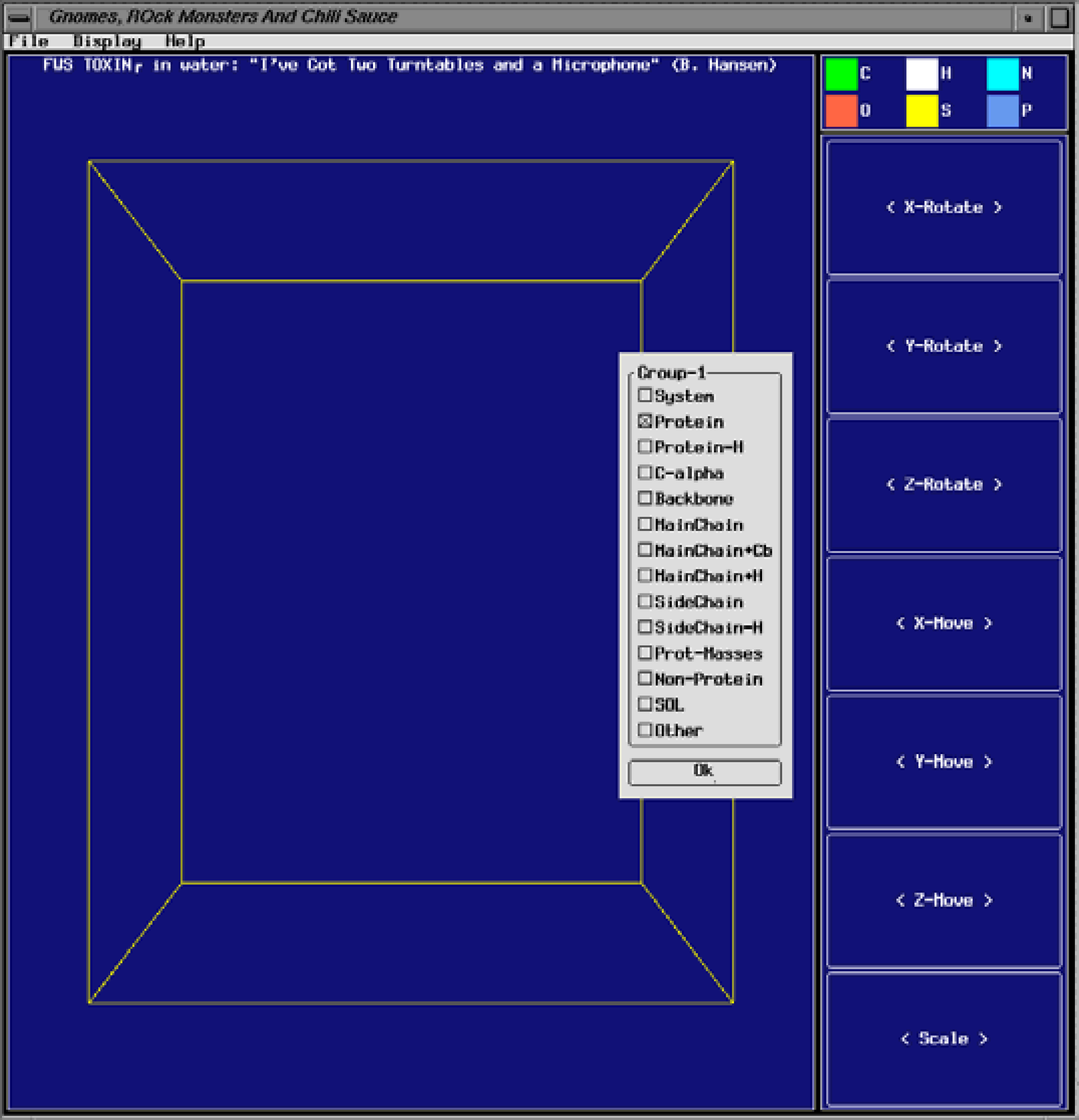
1. ngmx查看轨迹
很多时候, 我们需要粗略地查看一下模拟轨迹, 以确定模拟过程中没有出现明显的问题. 可以用GROAMCS自带的ngmx来快速查看轨迹. 需要注意的是, 在安装GROMACS时, 一般不会安装ngmx, 所以这个命令在你的机器上很可能无法使用.
gmx-4.x: ngmx -f npt-nopr.trr -s npt-nopr.tpr
gmx-5.x: gmx ngmx -f npt-nopr.trr -s npt-nopr.tpr
当查看器启动后, 将看到一个多选项的对话框. 选择标protein的多选框, 点击OK.
选择protein可以只显示蛋白质分子, 而隐藏盒子中的水分子.
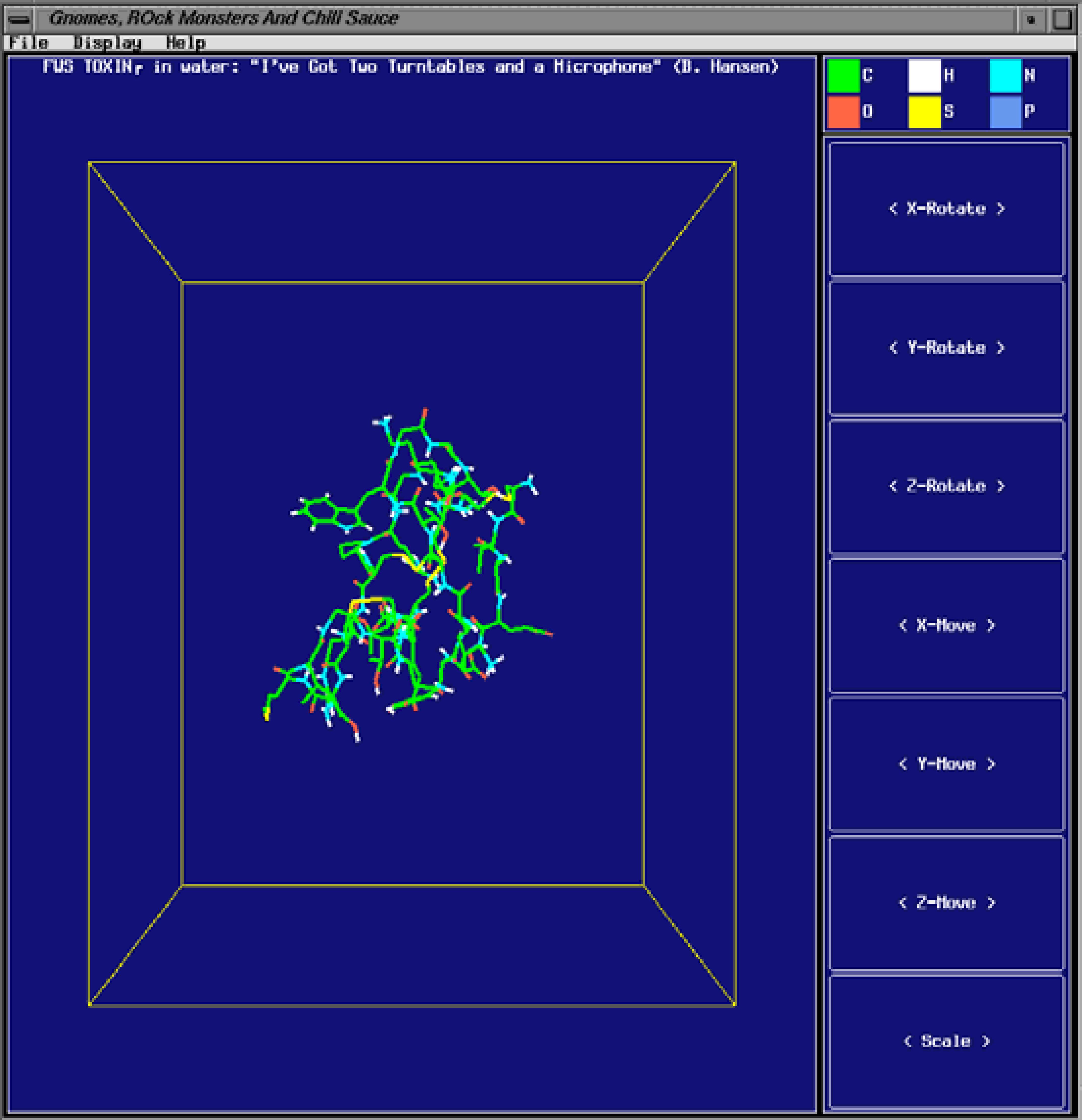
用X-Rotate上下旋转盒子(鼠标左键向上, 右键向下), 用Y-Rotate左右旋转盒子(左键向左, 右键向右).
最下面的Scale可用来放大或缩小视图(左键放大, 右键缩小).
要查看体系中的其它组, 点击Display->Filter, 会出现初始对话框, 供选择另外的索引组(如backbone)
要查看模拟轨迹动画, 点击Display->Animate. 动画播放控制在窗口的底部.
点击中间的箭头按钮逐帧观看, 点向前的双箭头观看整个轨迹动画, 点暂停按钮停止动画. 点向左的双箭头按钮重置动画.
不幸的是, File菜单下的save as pdb还不能用. 因此, 查看并保存*.pdb文件最好的方法是用VMD, 它学术免费, 在unix和Windows下都可以运行.
使用VMD查看轨迹的命令为
vmd em-sol.gro npt-nopr.xtc &
可以对蛋白质, 水和离子使用不同的表示模式. 要查看轨迹动画, 点击右下角的play forward按钮.
2. g_energy抽取性质数据
此命令可用于抽取能量输出文件中的数据, 如动能, 势能, 压力, 体积, 密度等, 以用于作图.
gmx-4.x: g_energy -f npt-nopr.edr -o enrg-npt.xvg
gmx-5.x: gmx energy -f npt-nopr.edr -o enrg-npt.xvg
运行上面的命令, 你将看到如下提示(gmx-4.x, 你看到的可能不同):
Select the terms you want from the following list by
selecting either (part of) the name or the number or a combination.
End your selection with an empty line or a zero.
-------------------------------------------------------------------
  1  Angle            2  Proper-Dih.      3  Improper-Dih.    4  LJ-14
  5  Coulomb-14       6  LJ-(SR)          7  Disper.-corr.    8  Coulomb-(SR)
  9  Coul.-recip.    10  Potential       11  Kinetic-En.     12  Total-Energy
 13  Temperature     14  Pres.-DC        15  Pressure        16  Constr.-rmsd
 17  Box-X           18  Box-Y           19  Box-Z           20  Volume
 21  Density         22  pV              23  Enthalpy        24  Vir-XX
 25  Vir-XY          26  Vir-XZ          27  Vir-YX          28  Vir-YY
 29  Vir-YZ          30  Vir-ZX          31  Vir-ZY          32  Vir-ZZ
 33  Pres-XX         34  Pres-XY         35  Pres-XZ         36  Pres-YX
 37  Pres-YY         38  Pres-YZ         39  Pres-ZX         40  Pres-ZY
 41  Pres-ZZ         42  #Surf*SurfTen   43  Box-Vel-XX      44  Box-Vel-YY
 45  Box-Vel-ZZ                          46  Coul-SR:Protein-Protein
 47  LJ-SR:Protein-Protein               48  Coul-14:Protein-Protein
 49  LJ-14:Protein-Protein               50  Coul-SR:Protein-non-Protein
 51  LJ-SR:Protein-non-Protein           52  Coul-14:Protein-non-Protein
 53  LJ-14:Protein-non-Protein           54  Coul-SR:non-Protein-non-Protein
 55  LJ-SR:non-Protein-non-Protein       56  Coul-14:non-Protein-non-Protein
 57  LJ-14:non-Protein-non-Protein       58  T-Protein
 59  T-non-Protein                       60  Lamb-Protein
 61  Lamb-non-Protein
若要抽取能量和温度数据, 可键入10 11 12 13并 回车两次 , 得到一个平均势能及其误差(gmx-4.x)
Statistics over 500001 steps [ 0.0000 through 1000.0000 ps ], 4 data sets
All statistics are over 5001 points

Energy                      Average   Err.Est.       RMSD  Tot-Drift
-------------------------------------------------------------------------------
Potential                   -176225         13     417.02    80.6394  (kJ/mol)
Kinetic En.                 31467.9        5.6    275.731   0.780693  (kJ/mol)
Total Energy                -144758         13    492.513    81.4195  (kJ/mol)
Temperature                 299.932      0.053    2.62809 0.00744002  (K)
gmx-5.x
Statistics over 500001 steps [ 0.0000 through 1000.0000 ps ], 4 data sets
All statistics are over 5001 points
Energy                      Average   Err.Est.       RMSD  Tot-Drift
-------------------------------------------------------------------------------
Potential                   -173825         20    432.623   -85.8249  (kJ/mol)
Kinetic En.                 31031.6        6.5    299.416    -33.179  (kJ/mol)
Total Energy                -142793         26    556.977   -119.003  (kJ/mol)
Temperature                 300.129      0.063    2.89586  -0.320896  (K)
gcq#155: "I Am a Wonderful Thing" (Kid Creole)
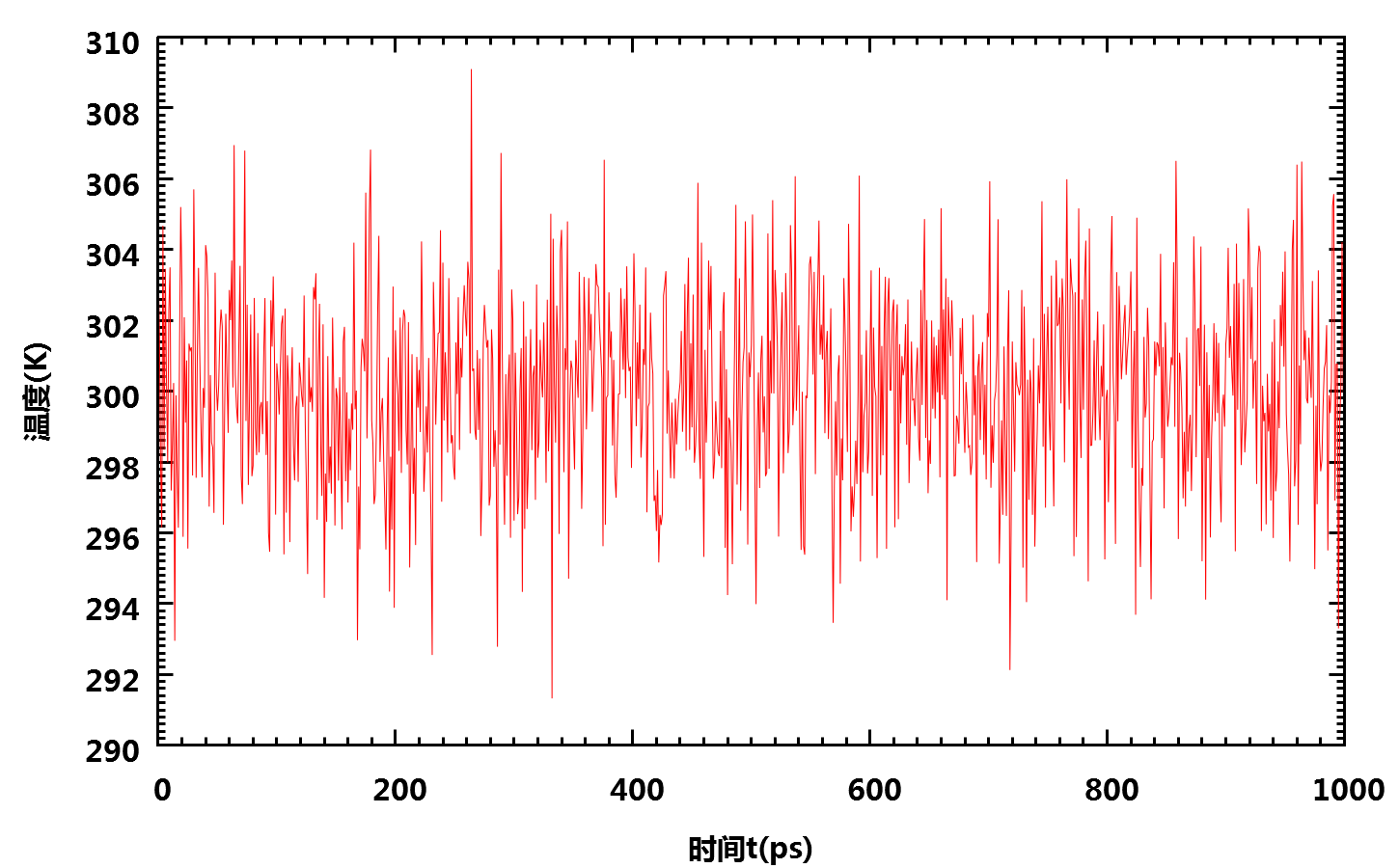
上面命令中的-o选项指定了数据的输出文件(*.xvg), 它是一个文本文件, 可以用Xmgr或Grace打开(只能在Linux和unix下使用),
xmgrace -nxy enrg-npt.xvg
Windows下有一个类似的qtgrace, 可作为Grace的替代品. 如果没有Xmgr或Grace, 在进行一些小的改动后也可以作为空格分隔文件导入Microsoft Excel作图. 当然, 也可以使用其他你熟悉的数据作图软件, 如Origin, gnuplot等. 下面是模拟过程中温度的变化图.
3. g_confrms比较构象差异
要比较模拟完成后的结构与初始PDB文件中结构的差异, 可使用g_confrms命令(用g_confrms -h查看详细信息).
gmx-4.x: g_confrms -f1 1OMB.pdb -f2 npt-nopr.gro -o fit.pdb
gmx-5.x: gmx confrms -f1 1OMB.pdb -f2 npt-nopr.gro -o fit.pdb
-f1和-f2指定需要进行比较的两个分子结构, -o指定叠合后分子结构的输出文件, fit.pdb包含两个分子结构的文件, 还可以使用-n1和-n2指定索引文件, 以选择用于叠合的原子.
运行命令后会提示选择一个组, 两次都选择4 (Backbone). 程序会对两个结构进行最小二乘拟合, 计算其RMSD值, 并输出结构文件(fit.pdb), 其中包含了叠合后的两个结构.
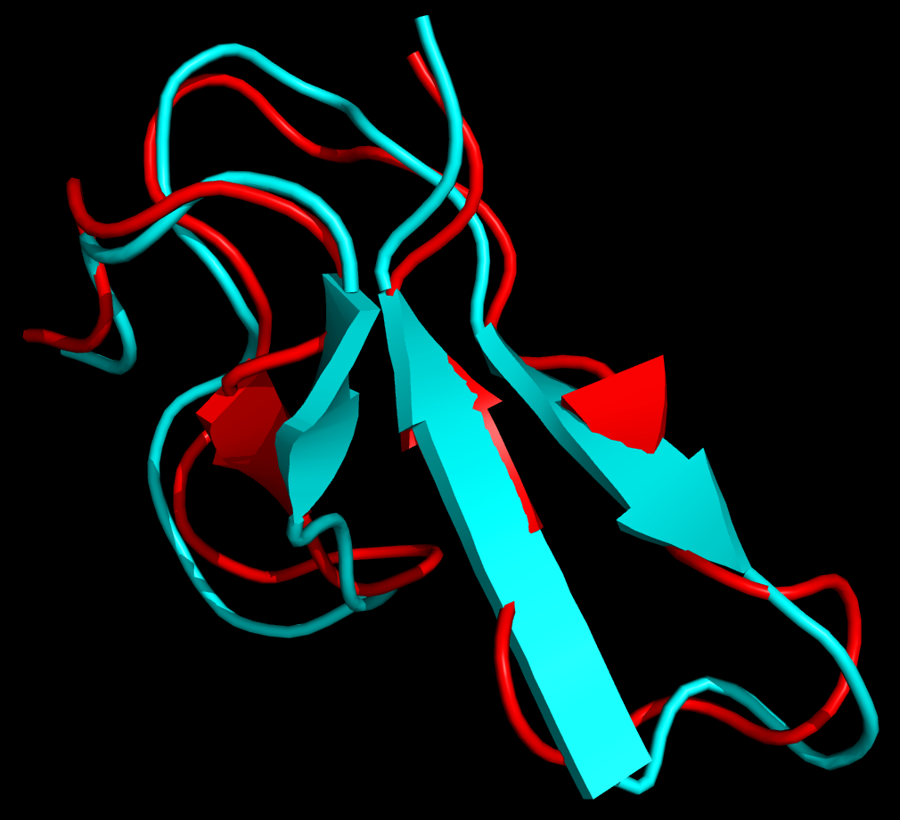
说明: 也可以使用editconf将两个结构转换为PDB文件, 然后都加载到PyMOL中, 使用align命令进行叠合.
【陈孙妮 补充说明】命令gmx confrms -f1 1OMB.pdb -f2 npt-nopr.gro -o fit.pdb得不到预期结果, 即fit.pdb中只有model1. 应对npt-nopr.gro进行处理, 去掉溶剂及离子, 则fit.pdb可以出现model1及model2.
测试结果如下(npt-nopr-h.gro是值去掉水及溶剂的npt-nopr.gro)
| 测试 | f1 | f2 | fit.pdb结果 |
|---|---|---|---|
| 1 | 1omb.pdb | npt-nopr.gro | 没有合并 |
| 2 | fws.gro | npt-nopr-h.gro | 跟图一样, 有二级结构, 但是是以两帧的形式存在,而不是并起来的 |
| 3 | 1omb.pdb | npt-nopr-h.gro | 跟图不一样, 无二级结构, 以两帧的形式存在, 而不是并起来的 |
| 4 | fws.pdb | npt-nopr-h.gro | 跟图不一样, 无二级结构, 以两帧的形式存在, 而不是并起来的 |
4. g_covar计算平均结构
g_covar命令可计算协方差矩阵(参见手册), 也可用于根据模拟轨迹计算平均结构. 如果要计算1 ns模拟轨迹中后200 ps的平均结构, 可使用
gmx-4.x: g_covar -f npt-nopr.xtc -s npt-nopr.tpr -b 801 -e 1000 -av npt-nopr_avg.pdb
gmx-5.x: gmx covar -f npt-nopr.xtc -s npt-nopr.tpr -b 801 -e 1000 -av npt-nopr_avg.pdb
注意, 平均结构往往比较粗糙, 需要进一步进行能量最小化.
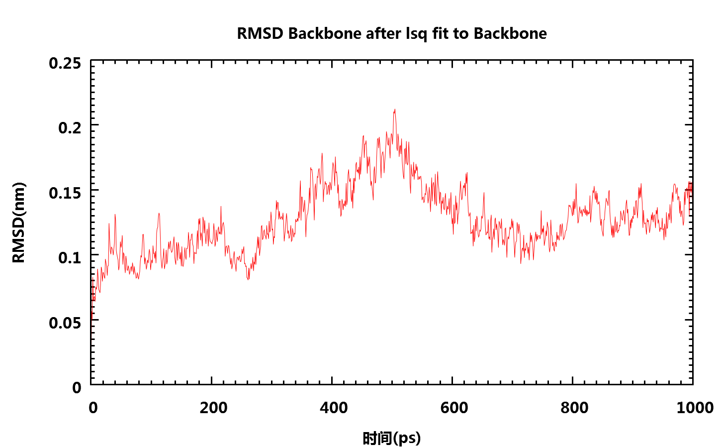
5. g_rms与g_rmsdist计算根均方偏差RMSD
这两个程序用于计算结构的RMSD值, 它可用于查看模拟的收敛性和蛋白的稳定性. 用g_rms计算模拟过程中的结构与初始结构的RMSD:
gmx-4.x: g_rms -s npt-nopr.tpr -f npt-nopr.xtc -o fws-bkbone-rmsd.xvg
gmx-5.x: gmx rms -s npt-nopr.tpr -f npt-nopr.xtc -o fws-bkbone-rmsd.xvg
提示时选择4 (Backbone)
程序会对结构进行最小二乘拟合并给出RMSD随时间的变化.
g_rmsdist命令可计算原子之间距离变化的RMSD:
gmx-4.x: g_rmsdist -s npt-nopr.tpr -f npt-nopr.xtc -o distrmsd.xvg
gmx-5.x: gmx rmsdist -s npt-nopr.tpr -f npt-nopr.xtc -o distrmsd.xvg
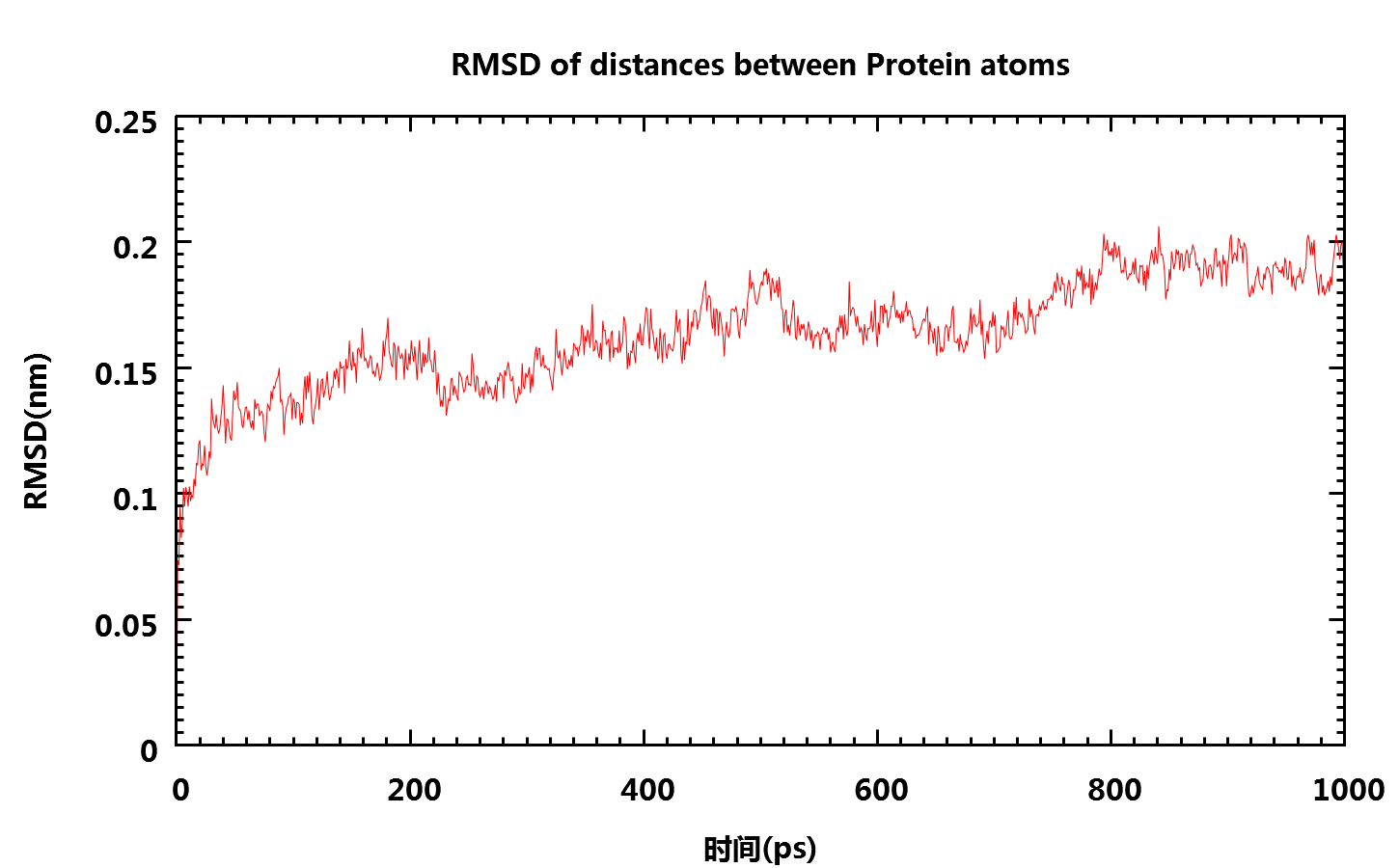
说明: 上面两个命令也可以使用索引文件选择需要计算的原子.
6. g_rmsf计算根均方涨落RMSF和温度因子
g_rmsf程序用于计算原子位置的根均方波动(RMSF). 均方根涨落的公式如下:
其中 $\bi r_t$ 为某一个时刻的构象, $\bi r_\text{ref}$ 为参考构象, $T$ 为总时间. RMSF和RMSD都是表征结构变化的量, 两者方程相似, 功能相似. 区别在于RMSD是对原子总数的平均, RMSF是对时间的平均. 在GROMACS中, g_rms得到的是随时间变化的曲线, g_rmsf得到的是随原子序号变化的曲线(可使用-res选项得到随氨基酸残基变化的曲线).
与g_covar类似, g_rmsf也可用于计算平均结构, 而且计算更快. 在实际研究中, 通常不需要计算整个轨迹的平均结构, 只需要计算达到平衡后后的平均结构, 可根据RMSD图(由g_rms计算)选择一个结构比较稳定的时间范围. 例如, 计算后500 ps范围内的平均结构, 可使用如下命令:
gmx-4.x: g_rmsf -s npt-nopr.tpr -f npt-nopr.xtc -b 500 -o fws-rmsf.xvg -ox fws-avg.pdb
gmx-5.x: gmx rmsf -s npt-nopr.tpr -f npt-nopr.xtc -b 500 -o fws-rmsf.xvg -ox fws-avg.pdb
提示时选择1 (Protein)回车即可. 注意, 平均结构往往比较粗糙, 需要进一步进行能量最小化.
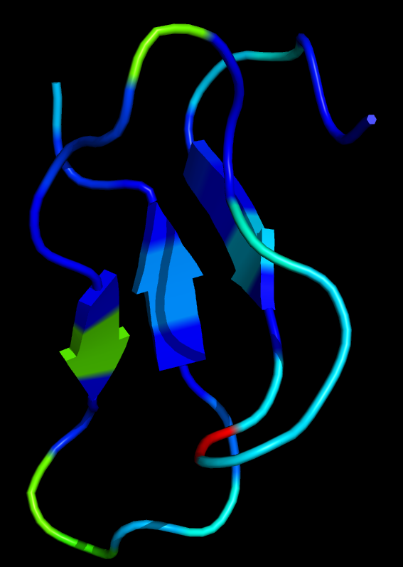
g_rmsf也可用于计算每个残基的温度因子, 得到的温度因子可以和X射线晶体结构的温度因子进行比较.
gmx-4.x: g_rmsf -s npt-nopr.tpr -f npt-nopr.xtc -o fws-rmsf.xvg -ox fws-avg.pdb -res -oq fws-bfac.pdb
gmx-5.x: gmx rmsf -s npt-nopr.tpr -f npt-nopr.xtc -o fws-rmsf.xvg -ox fws-avg.pdb -res -oq fws-bfac.pdb
提示时选择1 Protein, 回车.
将得到的bfactors.pdb载入PyMOL, 依次点击Hide->everything, Show->cartoon, Color->spectrum->b-factors, 或利用下面的PyMOL脚本处理得到的文件fws-bfac.pdb:
pymol bfactors.pdb
hide everything
show cartoon
spectrum b
若要指定温度因子的最大截断值, 可使用
Q = XXX
cmd.alter("all", "q = b > Q and Q or b")
spectrum q
其中的XXX为温度因子的最大截断值.
进行光线追踪后保存为图片, 或使用下面的命令:
ray 1200,1200
png bfac.png, dpi=300
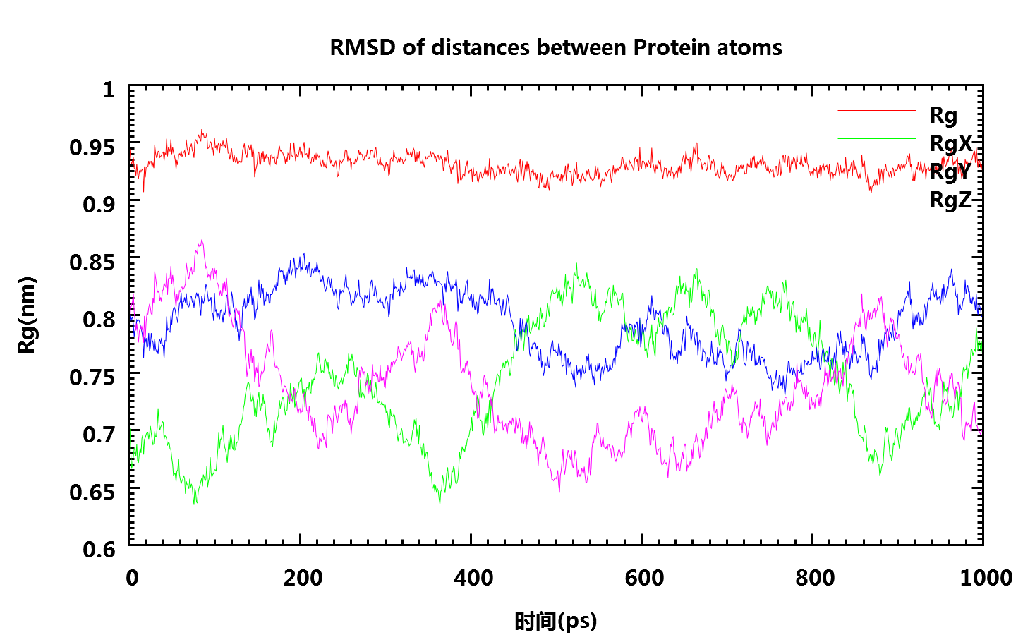
7. g_gyrate计算回旋半径
回旋半径取决于某(些)原子质量与分子重心的关系, 可用于表征蛋白质结构的密实度.
gmx-4.x: g_gyrate -s npt-nopr.tpr -f npt-nopr.xtc -o fws-gyrate.xvg
gmx-5.x: gmx gyrate -s npt-nopr.tpr -f npt-nopr.xtc -o fws-gyrate.xvg
选择1 Protein并回车.
8. g_sas计算溶剂可及表面积
氨基酸残基的疏水性是影响蛋白质折叠的重要因素, 溶剂可及表面积(SASA)是描述蛋白质疏水性的重要参数. 可利用g_sas计算蛋白质的溶剂可及表面积:
gmx-4.x: g_sas -s npt-nopr.tpr -f npt-nopr.xtc -o area.xvg -or resarea.xvg -oa atomarea.xvg
gmx-5.x: gmx sasa -s npt-nopr.tpr -f npt-nopr.xtc -o area.xvg -or resarea.xvg -oa atomarea.xvg
提示时选择1 (Protein)并回车.
9. do_dssp计算二级结构
do_dssp程序可计算模型的二级结构, 但前提是你的电脑中已经安装了dssp程序.
gmx-4.x: do_dssp -s npt-nopr.tpr -f npt-nopr.xtc -o fws-ss.xpm
gmx-5.x: gmx do_dssp -s npt-nopr.tpr -f npt-nopr.xtc -o fws-ss.xpm
提示时选择1 (Protein)并回车.
值得注意的是, 由于do_dssp的初衷是在Linux系统下运行, 所以无法在Windows下运行, 需要修改源代码才能达到在Windows下运行的目的.
可以用xpm2ps命令将得到的xpm文件转换为eps格式
gmx-4.x: xpm2ps -f fws-ss.xpm -o fws-ss.eps
gmx-5.x: gmx xpm2ps -f fws-ss.xpm -o fws-ss.eps
然后再使用ImageMagick程序的convert命令将eps文件转换为png图片格式或其他图片格式(也可使用Gimp程序或Windows下的IrfanView程序).
convert fws_ss.eps fws_ss.png
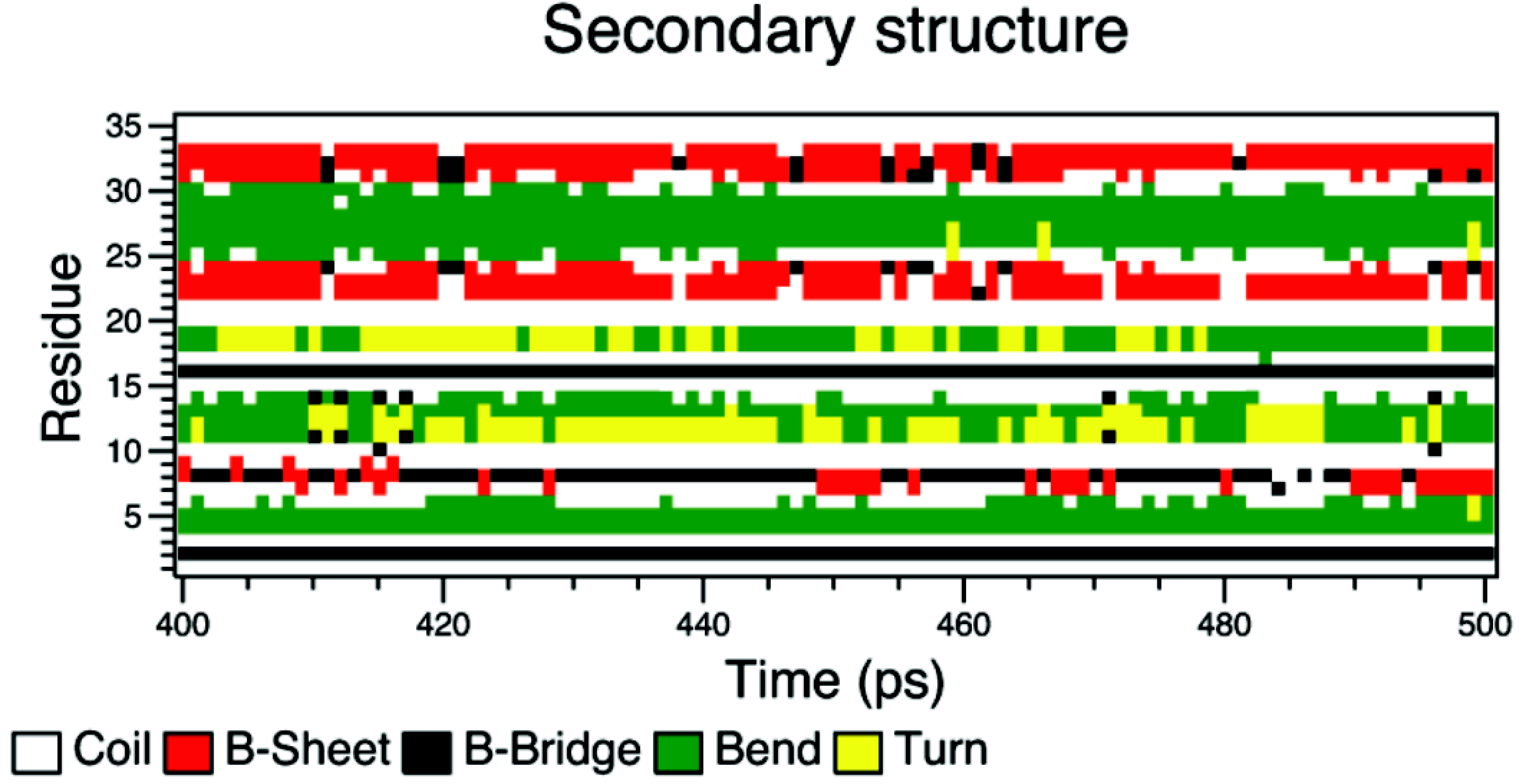
上面的dssp图中, y轴为残基编号, x轴为模拟时间(ps). 我们从中可以看到3个红色区域, 代表3个beta片层. 中间的较短区是最不稳定的, 这和前面温度因子的计算结果相符.
10. g_hbond统计氢键
g_hbond程序可用于计算模拟过程中分子间或组间的氢键数目以及氢键距离或角度的分布.
gmx-4.x: g_hbond -s npt-nopr.tpr -f npt-nopr.xtc -num fws_hnum.xvg
gmx-5.x: gmx hbond -s npt-nopr.tpr -f npt-nopr.xtc -num fws_hnum.xvg
提示时, 根据需要选择要分析的组. 一般选择(Protein)和(Water).
GROAMCS中氢键的默认判断标准如下
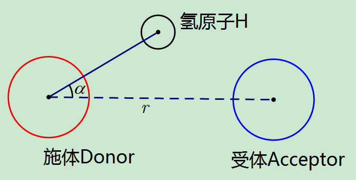
你可以使用-r和-a选项设定其它阈值. 默认地, g_hbond计算施体受体距离 $r_\text{DA}$, 可以用-da no选项设置为计算 $r_\text{HA}$ 距离.
11. g_saltbr分析盐桥
g_saltbr程序可用于分析模拟中残基间的盐桥. 程序会输出一系列xvg文件. 给出-/-, +/-(最关注的)和+/+残基间的距离.
gmx-4.x: g_saltbr -s npt-nopr.tpr -f npt-nopr.xtc
gmx-5.x: gmx saltbr -s npt-nopr.tpr -f npt-nopr.xtc
12. g_cluster分析团簇
g_cluster可使用各种方法进行团簇分析. 示例如下:
gmx-4.x: g_cluster -s npt-nopr.tpr -f npt-nopr.xtc -dm rmsd-matrix.xpm -dist rms-distribution.xvg -o clusters.xpm -sz cluster-sizes.xvg -tr cluster-transitions.xpm -ntr cluster-transitions.xvg -clid cluster-id-overtime.xvg -cl clusters.pdb -cutoff 0.25 -method gromos
gmx-5.x: gmx cluster -s npt-nopr.tpr -f npt-nopr.xtc -dm rmsd-matrix.xpm -dist rms-distribution.xvg -o clusters.xpm -sz cluster-sizes.xvg -tr cluster-transitions.xpm -ntr cluster-transitions.xvg -clid cluster-id-overtime.xvg -cl clusters.pdb -cutoff 0.25 -method gromos
使用下面的PyMOL脚本处理得到的文件
pymol clusters.pdb
split_states clusters
delete clusters
dss
show cartoon
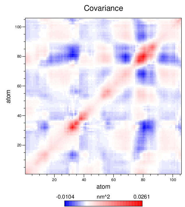
13. g_covar进行主成分分析
主成分分析PCA(Principal Components Analysis)方法可以帮助我们确定哪些运动方式对蛋白质的整个动力学贡献最大. 在含有N个原子的体系中, 存在3N-6个可能的内部运动方式(需要6个自由度来描述体系的外部转动和平动). 对PCA分析, 我们主要关心蛋白质骨架上的原子.
gmx-4.x: g_covar -s npt-nopr.tpr -f npt-nopr.xtc -o eigenval.xvg -v eigenvect.trr -xpma covara.xpm
gmx-5.x: gmx covar -s npt-nopr.tpr -f npt-nopr.xtc -o eigenval.xvg -v eigenvect.trr -xpma covara.xpm
对叠合和分析都选择组4 (Protein backbone)
使用xpm2ps制作原子协方差矩阵的图片, 其中使用-do选项会输出一个配置文件, 用于修改绘图的设置(坐标轴标题, 图例等).
gmx-4.x: xpm2ps -f covara.xpm -o covara.eps -do covara.m2p
gmx-5.x: gmx xpm2ps -f covara.xpm -o covara.eps -do covara.m2p
使用ghostview(或PhotoShop)来查看得到的图片(gv covara.eps). 使用xpm2ps -rainbow选项来采用其他的颜色方案.
典型的情况, 只有非常少的几个本征矢量(涨落模式)对蛋白质的整体运动有显著贡献. 要查看最主要的模式(1), 可使用下面的命令:
gmx-4.x: g_anaeig -v eigenvec.trr -s npt-nopr.tpr -f npt-nopr.xtc -first 1 -last 1 -nframes 100 -extr fws-ev1.pdb
gmx-5.x: gmx anaeig -v eigenvec.trr -s npt-nopr.tpr -f npt-nopr.xtc -first 1 -last 1 -nframes 100 -extr fws-ev1.pdb
分析二维本征矢量投影, 可使用
gmx-4.x: g_anaeig -s npt-nopr.tpr -f npt-nopr.xtc -first 1 -last 2 -2d proj-1-2.xvg
gmx-5.x: gmx anaeig -s npt-nopr.tpr -f npt-nopr.xtc -first 1 -last 2 -2d proj-1-2.xvg
14. g_angle进行二面角主成分分析
我们将创建一个索引文件来研究涉及残基MET29, ILE30, GLY31的4个二面角(2个phi, 2个psi). 使用VMD打开pr.gro或md.gro挑选与每个二面角对应的4个原子的索引号. 将文件命名为dangle.ndx.
gmx-4.x: g_angle -f npt-nopr.xtc -n dangle.ndx -or dangle.trr -type dihedral
gmx-5.x: gmx angle -f npt-nopr.xtc -n dangle.ndx -or dangle.trr -type dihedral
手动将(2*N/3)个原子写入covar.ndx中, 其中N为二面角的数目. 注意到g_angle的输出可以帮助你. 在g_angle的输出中你会发现需要三个原子位置的行.
共有4个二面角, 需要三个原子位置的cos/sin
[ test ] 1 2 3
创建一个辅助的gro文件用于g_covar分析
trjconv -s ../md.tpr -f dangle.trr -o resiz.gro -n covar.ndx -e 0
使用下面的命令进行g_covar分析
g_covar -f dangle.trr -n covar.ndx -ascii -xpm -nofit -nomwa -noref -s resiz.gro
检查第一个本征矢量的投影
g_anaeig -v eigenvec.trr -f dangle.trr -s resiz.gro -first 1 -last 1 -proj proj-1
当提示时, 选择0 (System).
检查本征矢量1和本征矢量2的二维投影
g_anaeig -v eigenvec.trr -f dangle.trr -s resiz.gro -first 1 -last 2 -2d 2dproj_1_2.xvg
使用g_analyze检查本征矢量1与其投影的余弦含量, 例如
g_analyze -f proj1.xvg -cc proj1-cc.xvg
当余弦含量接近于1时, 体系中的大尺度运动无法与随机扩散区分开来[8]. 对本征矢量1, 我们体系二面角的余弦含量大约为0.11, 可接受.
使用g_sham程序来查看自由能形貌:
g_sham -f 2dproj_1_2.xvg -ls gibbs.xpm -notime
xpm2ps -f gibbs.xpm -o gibbs.eps -rainbow red
参考文献
- Hess, B., et al., GROMACS 4: Algorithms for highly efficient, load-balanced, and scalable molecular simulation. J. Chem. Theor. Comp., 2008. 4(3): p. 435-447.
- Lindahl, E., B. Hess, and D. van der Spoel, GROMACS 3.0: a package for molecular simulation and trajectory analysis. J. Mol. Model, 2001. 7: p. 306-317.
- Lindorff-Larsen, K., et al., Improved side-chain torsion potentials for the Amber ff99SB protein force field. Proteins, 2010. 78: p. 1950-1958.
- Jorgensen, W., et al., Comparison of Simple Potential Functions for Simulating Liquid Water. J. Chem. Phys., 1983. 79: p. 926-935.
- Berendsen, H.J., J. Grigera, and T. Straatsma, The missing term in effective pair potentials. J. Phys. Chem., 1987. 91: p. 6269-6271.
- Weber, W., P.H. Hünenberger, and J.A. McCammon, Molecular Dynamics Simulations of a Polyalanine Octapeptide under Ewald Boundary Conditions: Influence of Artificial Periodicity on Peptide Conformation. J. Phys. Chem. B, 2000. 104(15): p. 3668-3575.
- Darden, T., D. York, and L. Pedersen, Particle Mesh Ewald: An N-log(N) method for Ewald sums in large systems. J. Chem. Phys., 1993. 98: p. 10089-10092.
- Essmann, U., et al., A smooth particle mesh ewald potential. J. Chem. Phys., 1995. 103: p. 8577-8592.
- Hess, B., et al., LINCS: A Linear Constraint Solver for molecular simulations. J. Comp. Chem., 1997. 18: p. 1463-1472.
- Maisuradze, G.G. and D.M. Leitner, Free energy landscape of a biomolecule in dihedral principal component space: sampling convergence and correspondence between structures and minima. Proteins, 2007. 67(3): p. 569-78.
- Hess, B. and N. van der Vegt, Hydration thermodynamic properties of amino acid analogues: a systematic comparison of biomolecular force fields and water models. J. Phys. Chem. B, 2006. 110(35): p. 17616-26.
- Berendsen, H.J.C., J.P.M. Postma, W.F. vanGunsteren, A. DiNola, and J.R. Haak, Molecular dynamics with coupling to an external bath. J. Chem. Phys., 1984. 81(8): p. 3584-3590.
- Bussi, G., D. Donadio, and M. Parrinello, Canonical sampling through velocity rescaling. J. Chem. Phys., 2007. 126(1): p. 14101.
- Kabsch, W. and C. Sander, A dictionary of protein secondary structure. Biopolymers, 1983. 22: p. 2577-2637.
附录: 更长时间模拟的参数文件
npt-longrun.mdp内容如下:
| npt-longrun.mdp | |
|---|---|
1 2 3 4 5 6 7 8 9 10 11 12 13 14 15 16 17 18 19 20 21 22 23 24 25 26 27 28 29 30 31 32 33 34 35 36 37 38 39 40 41 42 43 44 45 46 47 48 | ; RUN CONTROL PARAMETERS
integrator = md
tinit = 0 ; Starting time
dt = 0.002 ; 2 femtosecond time step for integration
nsteps = YYY ; Make it 50 ns
; OUTPUT CONTROL OPTIONS
nstxout = 250000 ; Writing full precision coordinates every
0.5 ns
nstvout = 250000 ; Writing velocities every 0.5 ns
nstlog = 5000 ; Writing to the log file every 10ps
nstenergy = 5000 ; Writing out energy information every 10ps
nstxtcout = 5000 ; Writing coordinates every 10ps
energygrps = Protein Non-Protein
; NEIGHBORSEARCHING PARAMETERS
nstlist = 5
ns-type = Grid
pbc = xyz
rlist = 1.0
; OPTIONS FOR ELECTROSTATICS AND VDW
coulombtype = PME
pme_order = 4 ; cubic interpolation
fourierspacing = 0.16 ; grid spacing for FFT
rcoulomb = 1.0
vdw-type = Cut-off
rvdw = 1.0
; Dispersion correction
DispCorr = EnerPres ; account for vdw cut-off
; Temperature coupling
Tcoupl = v-rescale
tc-grps = Protein Non-Protein
tau_t = 0.1 0.1
ref_t = 300 300
; Pressure coupling
Pcoupl = Parrinello-Rahman
Pcoupltype = Isotropic
tau_p = 2.0
compressibility = 4.5e-5
ref_p = 1.0
; GENERATE VELOCITIES FOR STARTUP RUN
gen_vel = no
; OPTIONS FOR BONDS
constraints = all-bonds
constraint-algorithm = lincs
continuation = yes ; Restarting after NPT without
position restraints
lincs-order = 4
lincs-iter = 1
lincs-warnangle = 30
|
评论
- 2016-06-03 14:59:27
franklinly0533您好,李老师,在《GROMACS教程:漏斗网蜘蛛毒素肽的溶剂化研究:Amber99SB-ILDN力场》中结果分析,1. ngmx查看轨迹,ngmx的初始启动对话框,ngmx查看蛋白质结构,这两个显示的结果已不能用ngmx命令了,我的电脑程序是5.1.2版本的。是不是可以改成:gmx nmtraj npt-nopr.trr -s npt-nopr.tpr gmx nmtraj npt-nopr.trr -s npt-nopr.tpr 在以下的命令中,- g_energy抽取性质数据
- g_confrms比较结构差异
- g_covar计算平均结构
- g_rms与g_rmsdist计算根均方偏差RMSD
- g_rmsf计算根均方涨落RMSF和温度因子
- g_gyrate计算回旋半径
- g_sas计算溶剂可及表面积
- do_dssp计算二级结构
- g_hbond统计氢键
- g_saltbr分析盐桥
- g_cluster分析团簇
- g_covar进行主成分分析
- g_angle进行二面角主成分分 均已经在5.1.2版本中消失了。均应该改为:
- gmx energy抽取性质数据
- gmx confrms比较结构差异
- gmx covar计算平均结构
- gmx rms与gmx rmsdist计算根均方偏差RMSD
- gmx rmsf计算根均方涨落RMSF和温度因子
- gmx gyrate计算回旋半径
- gmx sas计算溶剂可及表面积
- gmx do_dssp计算二级结构 10.gmx hbond统计氢键
- gmx saltbr分析盐桥
- gmx cluster分析团簇
- gmx covar进行主成分分析
- gmx angle进行二面角主成分分 另外,3. gmx confrms比较结构差异,我运行后得到的fit.pdb,结果用vmd软件打开,结果很乱,不是显示的蛋白结构。
-
2016-06-03 15:07:27
franklinly0533gmx do_dssp计算二级结构,gmx sas计算溶剂可及表面积。这两个程序运行了两遍,没有成功,还不知道哪里出现了问题,正在探究中。 -
2016-06-03 15:15:01
franklinly0533gmx saltbr分析盐桥,我的电脑运行结果如下: ……(注:结果行太多了,省略了) CG: CL4027-12422 Q: -1 Atoms: 12421 CG: CL4028-12423 Q: -1 Atoms: 12422 CG: CL4029-12424 Q: -1 Atoms: 12423 CG: CL4030-12425 Q: -1 Atoms: 12424 CG: CL4031-12426 Q: -1 Atoms: 12425 CG: CL4032-12427 Q: -1 Atoms: 12426 CG: CL4033-12428 Q: -1 Atoms: 12427 Reading frame 10 time 10.000 已杀死 这个说明是不是没有成功? -
2016-06-03 15:19:28
franklinly053312. gmx cluster分析团簇,这个我得到的结果如下: Error in user input: Invalid command-line options In command-line option -dm File ‘rmsd-matrix.xpm’ does not exist or is not accessible. For more information and tips for troubleshooting, please check the GROMACS website at http://www.gromacs.org/Documentation/Errors 命令行中的-dm 存在问题。rmsd-matrix.xpm不存在好像是由于前面有些步骤没有成功造成的哟。 -
2016-06-03 21:30:43
Jerkwin谢谢测试. 你能不能把你测试的结果发我一份Jerkwin@qq.com, 我好将教程更新到gmx 5.x? - 2016-10-06 11:29:35
CYM用http://jerkwin.github.io/9999/11/01/GROMACS%E7%A8%8B%E5%BA%8F%E7%BC%96%E8%AF%91/上提供的GROMACS 5.1.1双精度版时,发现在“第五步:向盒子中填充溶剂及离子并进行能量最小化”之后,fws.top文件会变成0字节,无法进行之后的第六步。本人电脑的操作系统是Windows 8.1。 -
2016-10-06 13:34:00
JerkwinWindows版本的gmx运行时由于权限问题可能导致无法自动更新top文件, 你需要自己手动将产生的一个名称中含有temp的临时文件复制到需要的top文件中, 直接将它重命名成需要的top文件也是可以的. - 2017-01-17 20:23:01
whtuLZ,pdb文件下不下来,请问在哪可以找到呢?谢谢。 - 2017-01-18 21:57:28
Jerkwin链接修复好了, 你再试试吧